Introduction to image processing - Radiometry
Sommaire
1 Introduction
For the following exercices, you need either Matlab or Scilab.
You need first to download the file TP.zip, to unzip it so that you have a directory named TP containing two subdirectories scilab_src (which contains a few necessary scilab commands for loading and displaying images) and im (which contains images needed in the TP).
If you use Scilab you should add scilab_src to the path by typing (replacing PATH by the correct path…) :
getd('/PATH/TP/scilab_src');
The comments are indicated by '%'in Matlab and by '//' in Scilab.
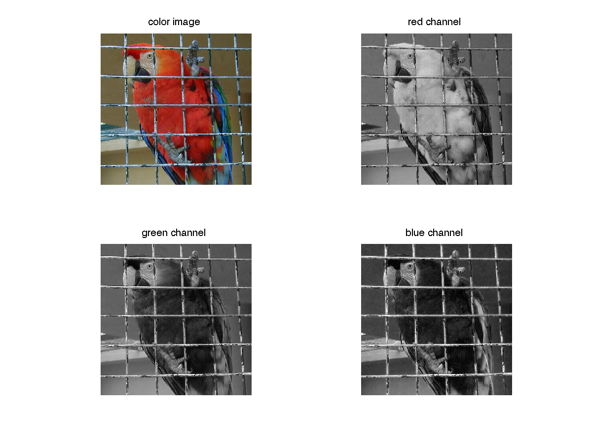
Load and display a color image. A color image \(u\) is made of three channels : red, green and blue. In Matlab and Scilab, a color image in \(\mathbb{R}^{N\times M}\) is stored as a \(N\times M\times 3\) matrix.
Scilab
imrgb = read_bmp_bg('im/parrot.bmp');  // load an image
[nrow,ncol,nchan]=size(imrgb);
ccview(imrgb); //display the color image
R = imrgb(:,:,1); G = imrgb(:,:,2); B = imrgb(:,:,3);
fview([R,G,B]); // display the three channels
Matlab
imrgb = imread('parrot.bmp');  % load an image
[nrow,ncol,nchan] = size(imrgb);  % image size
figure;
subplot(2,2,1); imshow(imrgb,[]), title('color image')
subplot(2,2,2), imshow(imrgb(:,:,1),[]), title('red channel');
subplot(2,2,3), imshow(imrgb(:,:,2),[]), title('green channel');
subplot(2,2,4), imshow(imrgb(:,:,3),[]), title('blue channel');
If you use Matlab, before most computations, it is important to convert an image to double (not necessary with Scilab).
imrgb = double(imrgb);
It might be useful to convert the color image to gray level. This can be done by averaging the three channels, or by computing another well chosen linear combination of the coordinates R, G and B. The rgb2gray function in the image processing toolbox computes \(0.2989 * R + 0.5870 * G + 0.1140 * B\).
imgray = sum(imrgb,3)/3;
Be careful with the function imshow(). If u is an image encoded in double, imshow(u) will display all values above 1 in white and all values below 0 in black. If the image u is encoded on 8 bits though, imshow(u) will display 0 in black and 255 in white. In order to scale u and use the full colormap, use the command imshow(u,[]).
2 Histograms and contrast enhancement
2.1 Computing histograms
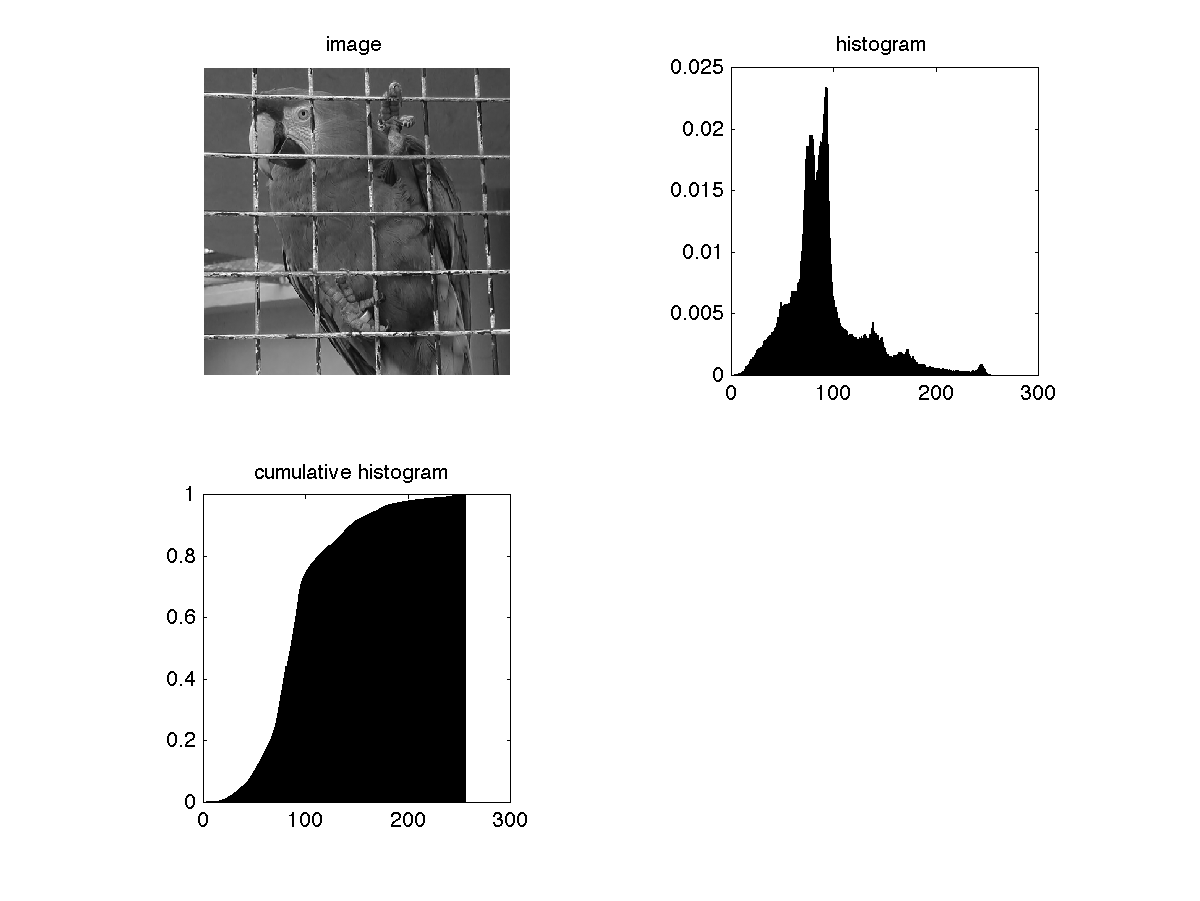
In the following, we compute and display the gray level histogram and the cumulative histogram of an image.
The cumulative histogram of a discrete image \(u\) is an increasing function defined on \(\mathbb{R}\) by $$H_u(\lambda)=\frac{1}{|\Omega|}\#{\{\textbf{x};\;u(\textbf{x})\leq \lambda\}}.$$ The histogram of \(u\) is the derivative of \(H_u\) in the sense of distributions.
imhisto = hist(imgray(:),[0:255]);  % or imhist(imgray(:),256); with Scilab
imhisto =imhisto/sum(imhisto);
imhistocum = cumsum(imhisto);
You can display both histograms with the command bar.
Matlab
figure; subplot(2,2,1); imshow(imgray,[]), title('image');
subplot(2,2,2), bar(imhisto), axis square, title('histogram');
subplot(2,2,3), bar(imhistocum), axis square, title('cumulative histogram');
2.2 Histogram equalization
If \(u\) is a discrete image and \(h_u\) its gray level distribution, histogram equalization consists in applying a contrast change \(g\) (increasing function) to \(u\) such that \(h_{g(u)}\) is as close as possible to a constant distribution. We can either use the function histeq of the image processing toolbox (use it on a 8bit image), or compute directly \(H_u(u)*255\).
imeq = imhistocum(uint8(imgray)+1)*255; % if imgray is between 0 and 1, multiply it by 255 before applying uint8
if you use Scilab, it is necessary to reshape the result with the command :
Scilab
imeq = matrix(imeq, nrow, ncol);
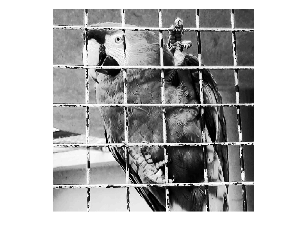
Display the result
figure, imshow(imeq,[]); % or fview(imeq) on Scilab;
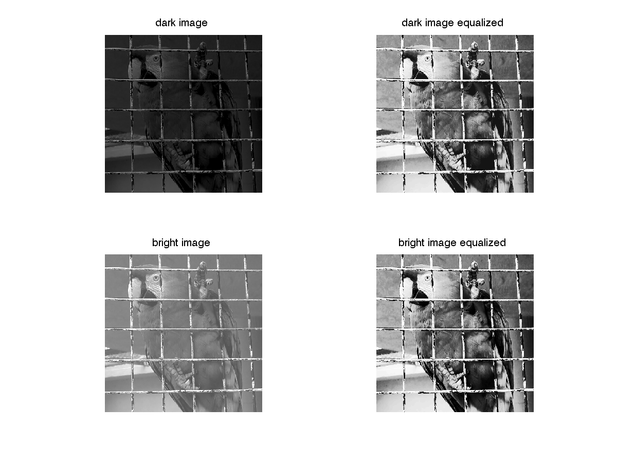
- Apply the histogram equalization to the images
parrot_bright.bmpandparrot_dark.bmpand plot the corresponding histograms and cumulative histograms. Comment the results and explain the observed differences.
2.3 Histogram specification
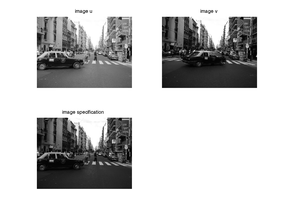
If \(u\) is a discrete image and \(h_u\) its gray level distribution, histogram specification consists in applying a contrast change \(g\) (an increasing function) to \(u\) such that \(h_{g(u)}\) is as close as possible to a target discrete probability distribution \(h_t\). Specification is particularly useful to compare two images of the same scene (in this case the target distribution is the histogram of the second image \(v\)).
- Histogram specification between two grey level images \(u\) and \(v\) can be computed easily by sorting the pixels of both images and by replacing each gray level in \(u\) by the gray level of similar rank in \(v\).
Matlab
u             = sum(double(imread('buenosaires3.bmp')),3)/3;             % use 'read_bmp_bg' with Scilab
v             = sum(double(imread('buenosaires4.bmp')),3)/3;
[u_sort,index_u]  = sort(u(:)); [v_sort,index_v]  = sort(v(:)); % use 'gsort' instead of sort with Scilab
uspecifv(index_u) = v_sort;
uspecifv = reshape(uspecifv,size(u));  % use 'matrix' instead of 'reshape' with Scilab
- Display the results.
Matlab
figure; subplot(2,2,1), imshow(u,[]), title('image u');
subplot(2,2,2), imshow(v,[]), title('image v');
subplot(2,2,3), imshow(uspecifv,[]), title('image specification');
linkaxes
- Translate the grey levels of \(u\) such that it has the same mean grey level than \(v\) and display the result. Is it similar to the specification of \(u\) on \(v\) ?
- Same question by applying an affine transform to \(u\) so that its mean and variance match the ones of \(v\).
2.4 Midway histogram
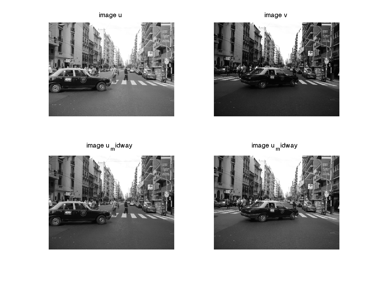
The Midway histogram between two histograms \(h_u\) et \(h_v\) is defined from it cumulative function \(H_{midway}\) : $$H_{midway}=\left( \frac{H_u^{-1}+H_v^{-1}}{2}\right)^{-1}.$$ The goal is to modify the contrast of both images \(u\) and \(v\) in order to give them the same intermediary grey level distribution.
Matlab (replace sort by gsort, reshape by matrix and imread by read_bmp_bg in Scilab)
u             = sum(double(imread('buenosaires3.bmp')),3)/3;
v             = sum(double(imread('buenosaires4.bmp')),3)/3;
[u_sort,index_u]  = sort(u(:));
[v_sort,index_v]  = sort(v(:));
u_midway(index_u) = (u_sort + v_sort)/2;
v_midway(index_v) = (u_sort + v_sort)/2;
u_midway = reshape(u_midway,size(u));
v_midway = reshape(v_midway,size(v));
Display the results.
Matlab
figure; subplot(2,2,1), imshow(u,[]), title('image u');
subplot(2,2,2), imshow(v,[]), title('image v');
subplot(2,2,3), imshow(u_midway,[]), title('image umidway');
subplot(2,2,4), imshow(v_midway,[]), title('image umidway');
2.5 Simple transformations
In this exercice, you are asked to perform simple transformations on an image and find out what happens on the corresponding histogram : thresholding, affine transformation, gamma correction.
2.6 Effect of Noise on histograms
In the following, we want to create different noisy versions of an image \(u\) and observe how the histogram \(h_u\) is transformed.
Gaussian noise Write a function adding a gaussian noise \(b\) to the image \(u\). An image of gaussian noise of mean \(0\) and of standard deviation \(\sigma\) is obtained with the command b=sigma*randn(nrow,ncol); on Matlab and b=sigma*rand(nrow,ncol,"normal"); on Scilab.
- Display the noisy image and its histogram for different values of \(\sigma\).
- What do you observe ? What is the relation between the histogram of \(u\) and the one of \(u+b\) ?
Uniform noise Same questions with \(b\) a uniform additive noise.
Impulse noise Let us recall that impulse noise destroy randomly a proportion \(p\) of the pixels in \(u\) and replace their values by uniform random values between \(0\) and \(255\). Mathematically, this can be modeled as \(u_b= (1-X)u+XY\), where \(X\) follows a Bernouilli law of parameter \(p\) and \(Y\) follows a uniform law on \(\{0,\dots 255\}\).
- Write a function adding impulse noise of parameter \(p\) to an image \(u\).
Hint : you can start by using the functionrandto create a table \(I\) of random numbers following the uniform law on \([0,1[\)
I = rand(size(U));
and then replace randomly \(p\%\) of the pixels (\(p\in[0,100]\)) of \(u\) by a random grey level
Ub = 255*rand(size(U)).*(I<p/100)+(I>=p/100).*U; - Display the noisy image and its histogram for different values of \(p\). What is the relation between the histogram of \(u\) and the one of \(u_b\) ?
3 Image Quantization
3.1 Quantization
Image quantization consists in reducing the set of grey levels \(Y = \{ y_0,\dots y_{n-1} \}\) or colors of an image \(u\) into a smaller set of quantized values \(\{q_0,\dots q_{p-1}\}\) (\(p < n\)). This operation is useful for displaying an image \(u\) on a screen that supports a smaller number of colors (this is needed with a standard screen if \(u\) is coded on more than 8 bits by channel).
A quantization operator \(Q\) is defined by the values \((q_i)_{i=0, \dots p-1}\) and \((t_j)_{j=0,\dots p}\) such that $$ t_0 \leq q_0 \leq t_1 \leq q_1 \leq \dots q_{p-1} \leq t_p,\text{ and } Q(\lambda)=q_i \text{ if } t_i \leq \lambda < t_{i+1}.$$
Uniform Quantization Uniform quantization consists in dividing the set \(Y\) in \(p\) regular intervals.
- Use uniform quantization on the grey level version of
lena(try different numbers \(K\) of grey levels) and display the result. For which value of \(K\) do you start to see a difference with the original image ?
for K=50:-1:1
uquantif = (floor(u*(K-1)/255)+0.5)*255/(K-1); % quantization on K=10 grey levels
imshow(uquantif,[]);
pause(0.1);
end

Histogram-based Quantization This consists in choosing \(t_i=\min \{\lambda; H_u(\lambda) \geq \frac{i}{p} \}\), and the \(q_i\) are defined as the barycenters of the intervals $[ti,ti+1].$
- Show that this boils down to an histogram equalization followed by a uniform quantization
- Apply this quantization on the grey level version of
lena.bmpand display the result. Same question on the limit value \(K\) for which we perceive a difference with the original image.
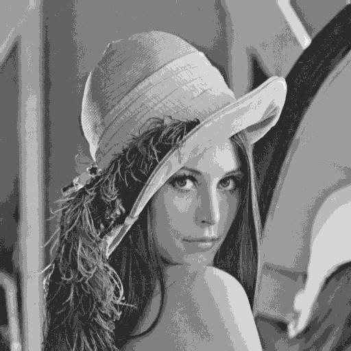
Lloyd-Max quantization This quantization consists in minimizing the least square error $$LSE((q_i)_{i=1\dots p-1},(t_i)_{i=1\dots p})= \sum_{i=0}^{p-1} \sum_{y_j \in [t_i,t_{i+1}[} h_i (y_j -q_i)^2.$$
- Write the optimality conditions that should be satisfied by the solution \(\{(\widehat{q_i}),(\widehat{t_i})\}\).
- Write a function which minimizes the least square error by alternatively minimizing in \((q_i)_{i=0, \dots p-1}\) and \((t_j)_{j=0,\dots p}\).
- Apply this quantization on the grey level version of
lena.bmpfor different values of \(K\) and display the result. Comment.
Quantization on 10 levels with Lloyd Max
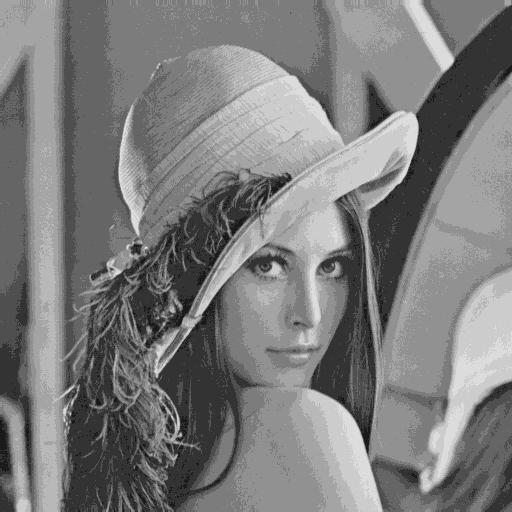
3.2 Dithering
Dithering consists in adding intentionnally noise to an image before quantization. For instance, it can be used to convert a grey level image to black and white in such a way that the density of white dots in the new image is an increasing function of the grey level in the original image. This is particularly useful for impression or displaying.
Let us explain how dithering works in the case of 2 grey levels (binarization). All grey levels smaller than a value \(\lambda\) are replaced by \(0\) and those greater than \(\lambda\) are replaced by \(255\). If we add a i.i.d. noise \(B\) of density \(p_B\) to \(u\) before the binarization, then at the pixel \(x\) we get $$P[u(x) + B(x) > \lambda] = P[B(x) > \lambda - u(x) ] = \int_{\lambda - u(x)}^{+\infty} p_B(s)ds,$$ which is an increasing function of the value \(u(x)\). The probability that \(x\) turns white in the dithered image is thus an increasing function of its original grey level.
- Perform dithering to reduce the number of grey levels of
lena.bmp. Compare the result with a quantization without dithering.

