Image segmentation with active contours
Table des matières
For the following exercices, you need Matlab. The subject of the following exercices is image segmentation. We denote by \(u_0\) the image we want to segment.
1 Introduction
The model of Chan and Vese is described in Chan, T. F., & Vese, L. (2001). Active contours without edges. Image processing, IEEE transactions on, 10(2), 266-277.
In this model, we segment an image \(u_0\) with a set of edges \(K\) by minimizing the energy \[F(K)=\lambda \mathcal{L}(K) + \alpha_{in} \int_{inside(K)} |u_0-c_{in}|^2+ \alpha_{out} \int_{outside(K)} |u_0-c_{out}|^2,\] where \(\mathcal{L}(K)\) is the length of the contour \(K\), \(c_{in}\) is the mean of \(u_0\) inside the \(K\) and \(c_{out}\) is the mean of \(u_0\) outside of \(K\) \[c_{in} = \frac{\int_{inside(K)} u(x)dx}{\int_{inside(K)}dx},\;\;\;\;\; c_2 = \frac{\int_{outside(K)} u(x)dx}{\int_{outside(K)} dx}.\]
2 Chan-Vese segmentation - Level set approach
Several approaches are possible to minimize this non convex energy. The first one consists in using a level set approach and to represent \(K\) as the zero level curve of a well chosen function \(\phi\). In order to minimize \(F\), \(\phi\) must follow the evolution equation \[\frac{\partial \phi}{\partial t}= \lambda \delta_{\epsilon}(\phi) \left[ div \left( \frac{\nabla \phi}{|\nabla \phi|} \right) -\alpha_{in} (u_0-c_{in})^2 +\alpha_{out} (u_0-c_{out})^2 \right],\] where \[div \left( \frac{\nabla \phi}{|\nabla \phi|}\right) = \frac{\phi_{xx}\phi_{y}^2 - 2 \phi_{x}\phi_{y}\phi_{xy}+ \phi_{yy}\phi_{x}^2}{(\phi_{x}^2+\phi_{y}^2)^{3/2}},\;\; c_{in} = \frac{\int u_0 \mathbf{1}_{\phi \geq 0 }}{\int \mathbf{1}_{\phi \geq 0 }},\;\;c_{out} = \frac{\int u_0 \mathbf{1}_{\phi < 0 }}{\int \mathbf{1}_{\phi < 0 }}.\] As proposed in the paper of Chan and Vese, we can regularize the Dirac distribution with \[\delta_{\epsilon}(\phi) = \frac{\epsilon}{\pi (\epsilon^2+\phi^2)}.\]
In order to implement the previous descent scheme, we will use the function 'imgradientxy' of Matlab with the option 'IntermediateDifference' to compute the first and second derivative of Phi. If you do not have access to the image processing toolbox, write yourself a function which computes these derivative.
- Read the image \(f\)
f = double(imread('im/magritte512.jpg'));
f = f(:,:,2);
f = f/max(f(:));

- Create the initial contour with the function roipoly
mask = roipoly(f);     % create a binary mask
mask = 2*mask - 1;     % put the mask on {-1,1}
figure;imshow(f,[]);hold on;
contour(mask,[0.5 0.5],'b');
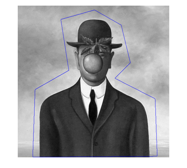
- Initialize the different parameters
dt = 0.1;       % Scheme step
eta = 0.01;     % Small value to avoid division by zero.
epsilon = 0.1;  % Epsilon used for the delta approximation
alpha_in = 1;   % fidelity terms
alpha_out = 1;
Phi = mask;
N = 1500;       % number of iterations
- Implement the Chan-Vese scheme
for k = 1:N
    %Compute the  derivatives
    [Phi_x,Phi_y] = imgradientxy(Phi,'CentralDifference');
    [Phi_xx,Phi_xy] = imgradientxy(Phi_x,'CentralDifference');
    [Phi_yx,Phi_yy] = imgradientxy(Phi_y,'CentralDifference');

    %Compute the values c_in and c_out
    c_in = sum((Phi>0).*f)/(eta+sum((Phi>0)));
    c_out = sum((Phi<0).*f)/(eta+sum((Phi<0)));

    %TV term = Num/Den
    divgrad_num = Phi_xx.*Phi_y.^2 - 2*Phi_x.*Phi_y.*Phi_xy + Phi_yy.*Phi_x.^2;
    divgrad_denom = (Phi_x.^2 + Phi_y.^2).^(3/2) + eta;
    divgrad = divgrad_num./divgrad_denom;

    %Update Phi
    Phi = Phi + dt*epsilon./(pi*(epsilon^2+Phi.^2)).*(divgrad  - alpha_in*(f-c_in).^2 + alpha_out*(f-c_out).^2);
end
- Display the results
figure;imshow(Phi>0,[]);hold on;
contour(mask,[0.5 0.5],'b'); contour(Phi>0,[0.5 0.5],'r');
legend('Initialisation','Final Result');
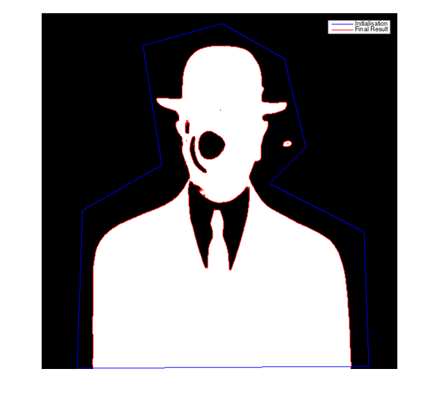
Image processing toolbox: activecontour function
The previous method is also implemented in the (faster) function activecontour of the Matlab image toolbox. You can for instance apply the Chan-Vese algorithm with 300 iterations with the command
ac = activecontour(f,mask,300,'Chan-Vese');
Observe that if you use the option 'edge' instead of 'Chan-Vese', the active contour scheme of Caselles-Kimmel-Sapiro is applied.
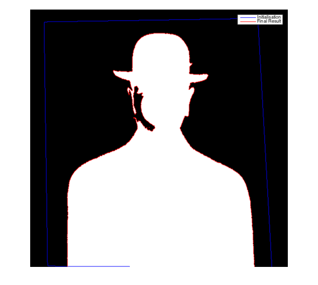
Display the results
figure;imshow(ac,[]);hold on;
contour(mask,[0.5 0.5],'b'); contour(ac,[0.5 0.5],'r');
legend('Initialisation','Final Result');
Observe that the result is not exactly the same as the one obtained with our implementation. How can you explain these differences ?
In the recent versions of Matlab, you can also use an interactive tool called imageSegmenter, which permits to see the animated contour along the iterations.
imageSegmenter(f)
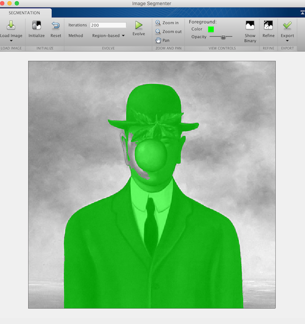
- Use one of the previous tools to segment the Magritte image. Is the result at convergence strongly dependent on the initialization ? Do the same experiment with the Caselles-Kimmel-Sapiro scheme.
- The Chan-Vese algorithm is also available as an IPOL demo (with animated segmentation evolutions).
3 Chan-Vese segmentation - Convexification
Another solution relies on the convexification of the energy. In the previous formulation, the contour \(K\) can be replaced by a binary function \(w:\Omega \longrightarrow \{0,1\}\) whose discontinuities correspond to \(K\). The energy becomes \[F(w)=\underbrace{\lambda \int_{\Omega} \|\nabla w\|}_{\lambda TV(w)} + \underbrace{\alpha_{in} \int_{\Omega} w|u_0-c_{in}|^2+ \alpha_{out} \int_{\Omega} (1-w)|u_0-c_{out}|^2}_{G(w)},\] where \[c_{in} = \frac{\int u w}{\int w},\; c_{out} = \frac{\int (1-w) u}{\int (1-w)}.\]
The function \(F\) is convex, but the minimization \[\min_{w:\Omega \rightarrow \{0,1\}} F(w) \;\;\;\;\;\; \;\;\;\;\;\; (*)\] is still not convex because the constraint \(\{0,1\}\) is not. However, this optimization problem can be convexified in \[\min_{w:\Omega \rightarrow [0,1]} F(w),\] and it can be shown that the minimizers of (*) are merely binarizations of the global minimizers of this last convex energy (see for instance [Bresson et al., 2007]).
Chambolle-Pock primal-dual algorithm The previous convex energy can be minimized for instance by using Chambolle-Pock primal-dual algorithm [Chambolle-Pock, 2011]. The code is very similar to the one we saw in the restoration exercices for the TV-L1 problem (see here).
We want to find a \([0,1]\) valued function which minimizes \[ G(w) + \lambda TV(w) = G(w) + F(Kw),\] where \[K =\lambda \nabla \;\;\text{and}\;\; G(w) = \int_{\Omega} w|u_0-c_{in}|^2+ \alpha_{out} \int_{\Omega} (1-w)|u_0-c_{out}|^2.\]
We write (with \(\iota_{\kappa}\) the characteristic function of the convex set \(\kappa\)) \[ TV(w) = \max_{p\in X\times X} <\nabla w, p >_X -\underbrace{\iota_{\kappa}(p)}_{F^*(p)}, \;\;\text{with}\;\; \kappa = \{\mathrm{div} p \;/ \;\max_{x\in\Omega}|p(x)| \leq 1\}.\]
The primal-dual algorithm for the segmentation problem can be written
- Initialization : choose \(\tau\), \(\sigma >0\), \((w^0,p^0)\)
- Iterations for \(n\geq 0\) : \begin{cases} p^{n+1} &=& \underbrace{\mathrm{prox}_{\sigma F^*}}_{\text{backward step}} \underbrace{(p^n + \sigma K \bar{w}^n)}_{\text{forward step}} \\ w^{n+1} &=& \mathrm{prox}_{\tau G} (w^n-\tau K^* p^{n+1})\\ \bar{w}^{n+1} &=& w^{n+1} + \theta (w^{n+1} - w^n) \end{cases}
The proximal operators \(\mathrm{prox}_{\sigma F^*}\) and \(\mathrm{prox}_{\tau G}\) are easy to compute in this case, \[\left(\mathrm{prox}_{\tau G}(w)\right)_{i,j} = w_{i,j} - \tau ((f_{i,j} - c_{out})^2 - (f_{i,j} - c_{in})^2);\] \[\left(\mathrm{prox}_{\sigma F^*}(p)\right)_{i,j} = \left(\pi_{\kappa}(p)\right)_{i,j} = \frac{p_{i,j}}{\max(1,|p_{i,j}|)}.\]
The convergence analysis in [Chambolle-Pock 2010] shows that the previous algorithm converges for \(\theta = 1\) if $$\tau\sigma.|||K|||^2 <1,\;\; \;\;\; \text{ i.e. } \;\; \;\;\tau\sigma.8\lambda^2 <1.$$
Read f
f = double(imread('magritte512.jpg'));
f = f(:,:,2);
f = f/max(f(:));
imshow(f);
Apply [Chambolle-Pock, 2010] with \(K=\lambda \nabla (\text{ thus } K^* = -\lambda \mathrm{div})\), \(F = \lambda ||.||_1\) and \(G\) chosen as above (choose \(\alpha_{in} = \alpha_{out} = 1\) for the sake of simplicity).
w=rand(size(f));                % initialisation of w
n=100;
p = zeros([size(f),2]);
lambda = 1;
tau   = 0.99/sqrt(8*lambda^2);  % see Chambolle Pock 2010
sigma = 0.99/sqrt(8*lambda^2);
wbar = w;                       %
theta = 1;

for k=1:n
    % proxF
    [gx,gy]  = grad_im(wbar);
    g = cat(3,gx,gy);
    p = p + lambda*sigma*g;
    normep = max(1,sqrt(p(:,:,1).^2+p(:,:,2).^2));
    p(:,:,1) = p(:,:,1)./normep;
    p(:,:,2) = p(:,:,2)./normep;

    % proxG
    d=div_champ(p(:,:,1),p(:,:,2));
    c0      = sum(sum(f.*w))/sum(sum(w));
    c1      = sum(sum(f.*(1-w)))/sum(sum(1-w));
    normext = (f - c0).^2;
    normint = (f - c1).^2;
    v = w+tau*(lambda*d - normext + normint);
    wnew = max(0,min(1,v));

    %extragradient step
    wbar = wnew+theta*(wnew-w);
    w = wnew;

end
Display the resulting segmentation and boundaries
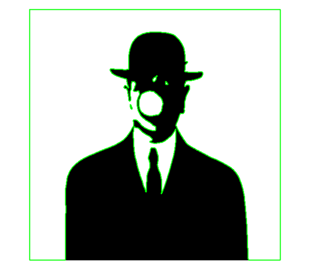
BW = w>0.5;                        % binarization
[B,L,N] = bwboundaries(BW);
figure; imshow(BW); hold on;       % display BW
for k=1:length(B),
    boundary = B{k};
    plot(boundary(:,2),boundary(:,1),'g','LineWidth',2);      % display the boundaries
end