Restoration of images corrupted with Gaussian noise
Table of Contents
Observation model
Let \(u: \Omega \to \RR\) be an (unobserved) intensity image defined on a discrete domain \(\Omega\) (a rectangular subset of \(\ZZ^2\)). Instead of \(u\) assume that a noisy (random) observation \(u_0\) is available, more precisely consider that
\[ \forall (x,y) \in \Omega, \quad u_0(x,y) = u(x,y) + n(x,y)\;, \]
where the \(n(x,y)\) are realizations of indenpendant Gaussian random variables with zero-mean and variance \(\sigma^2\).
Maximum A Posteriori: from Bayesian to variational framework
According to the observation model, the probability density function (p.d.f) is given by
\begin{equation} \label{eq:likelihood} % p(u_0 \,|\, u) = \prod_{(x,y) \in \Omega} \tfrac{1}{\sigma \sqrt{2\pi}} \, e^{-(u(x,y)-u_0(x,y))^2/2\sigma^2} % = \left(\tfrac{1}{\sigma \sqrt{2 \pi}}\right)^{|\Omega|} \, \exp{ \left( -\frac{\| u - u_0 \|_2^2}{2\sigma^2} \right) } \;. % \end{equation}Using the improper (discrete) \(\TV\) prior \(p(u) \propto e^{-\beta \TV(u)}\) (where \(\beta\) is a positive regularization parameter) and Equation \eqref{eq:likelihood}, we get thanks to the Bayes rule the posterior density
\begin{equation} \label{eq:posterior} % p(u \,|\, u_0) \propto p(u_0 \,|\, u) \, p(u) = \exp{\left(- \frac{\|u-u_0\|_2^2}{2\sigma^2} - \beta \TV(u) \right)} \;. % \end{equation}Note that notation \(\propto\) indicates an equality up to a global multiplicative constant (which depends on \(u_0\) but not of \(u\)).
The Maximum A Posteriori (MAP) consists in computing the image that maximizes the posterior density \(p(u \,|\,u_0)\), or equivalently that minimizes the convex energy \(-\log{p(u \, | \, u_0)}\). Finally the MAP approach boils down to the variational problem
\begin{equation} \label{eq:primal-rof} % \widehat{u}_\text{MAP} = \arg\, \min_{u \in \RR^\Omega} \tfrac{1}{2} \| u - u_0 \|_2^2 + \lambda \TV(u) \;, % \end{equation}where \(\lambda = \beta \sigma^2\) is a parameter that must be set by the user, it controls the tradeoff between data fidelity (the quadratic term) and regularity (the total variation term).
This variational problem was first proposed by Rudin, Osher and Fatemi (ROF) in [1].
Primal-dual reformulation
Recall the dual formulation of the discrete total variation (see here the page dedicated to the discrete total variation)
\[ \TV(u) = \max_{p \in \RRRR{\Omega}} \langle \nabla u , p \rangle \quad \text{subject to} \quad \|p\|_{\infty,2} \leq 1 \;, \]
where \(\|p\|_{\infty,2} = \max_{(x,y) \in \RR^\Omega} \|p(x,y)\|_2\).
Noting \(\delta\) the indicator function of the closed unit ball of the norm \(\|\cdot\|_{\infty,2}\), that is
\begin{equation} \forall p \in \RRRR{\Omega}, \quad \delta(p) = \left\{ \begin{array}{cl} 0 & \text{if } \|p\|_{\infty,2} \leq 1 \\ +\infty & \text{otherwise,} \end{array} \right. \end{equation}and replacing the \(\TV\) term by its dual formulation into equation \eqref{eq:primal-rof} we obtain a primal-dual (saddle-point) reformulation of problem \eqref{eq:primal-rof},
\begin{equation} \label{eq:primal-dual-rof} % \hat{u}_\text{MAP} = \arg \, \min_{u \in \RR^\Omega} \, \max_{p \in \RRRR{\Omega}} \tfrac{1}{2} \|u-u_0\|_2^2 + \langle \lambda \nabla u , p \rangle - \delta(p) \;, % \end{equation}that can be numerically solved thanks the Chambolle and Pock algorithm [3].
Computational procedure
The Chambolle and Pock algorithm
A solution of problem \eqref{eq:primal-dual-rof} can be numerically computed using the algorithm of Chambolle-Pock [3], which is designed to solve the generic saddle-point problem
\begin{equation} \label{eq:cp.primal-dual} \arg\,\min_{x \in X}\max_{y \in Y} ~ G(x) + \langle Kx , y \rangle - F^\star(y) \;. \end{equation}The algorithm is briefly presented on this page.
Taking \(X=\RR^\Omega\), \(Y=\RRRR{\Omega}\), \((x,y) = (u,p)\), \(F^\star(p) = \delta(p)\), \(G(u) = \tfrac{1}{2} \|u-u_0\|_2^2\) and \(K = \lambda \nabla\) into problem \eqref{eq:cp.primal-dual} allows to recover problem \eqref{eq:primal-dual-rof}.
Noting \(\divergence = -\nabla^*\) the opposite of the adjoint of the operator \(\nabla\) (in analogy with the continuous setting), we have \(K^* = -\lambda \divergence\), then the Chambolle and Pock algorithm applied to problem \eqref{eq:primal-dual-rof} boils down to Algorithm 1.
Chambolle-Pock resolvant algorithm for problem \eqref{eq:primal-dual-rof}.
Initialization: Choose \(\tau, \sigma > 0\), \(\theta \in [0,1]\), \(u^0 \in \RR^\Omega\), \(p^0 \in \RRRR{\Omega}\) and set \(\bar{u}^0 = u^0\).
Iterations (\(k \geq 0\)): Update \(u^k,p^k\) and \(\bar{u}^k\) as follows
\begin{eqnarray} p^{k+1} &=& \arg\,\min\limits_{\substack{p \in \RRRR{\Omega} }} ~ \tfrac{1}{2\sigma} \left\|p-(p^k+\sigma \lambda \nabla \bar{u}^k)\right\|_2^2 + \delta(p) \label{cp.dual} \\ u^{k+1} &=& \arg\,\min\limits_{\substack{u \in \RR^\Omega}} ~ \tfrac{1}{2\tau} \left\|u-\left(u^k +\tau \lambda \divergence p^{k+1} \right)\right\|_2^2 + \tfrac{1}{2} \| u - u_0\|_2^2 \label{cp.primal} \\ \bar{u}^{k+1} &=& u^{k+1} + \theta \left(u^{k+1}-u^{k}\right) \nonumber \end{eqnarray}\(~\)
The primal and dual updates (Equations \eqref{cp.primal} and \eqref{cp.dual}) can be computed in closed-form.
The dual update \eqref{cp.dual} boils down to the pointwise operations \[ % \forall (x,y) \in \Omega, \quad p^{k+1}(x,y) = \frac{p^k(x,y) + \sigma \lambda \nabla \bar{u}^k(x,y) }{\max { \left( 1 , \left|\, p^k(x,y) + \sigma \lambda \nabla \bar{u}^k(x,y) \,\right|_2 \right) }} \;, % \] and the primal update \eqref{cp.primal} boils down to the pointwise operations \[ \forall (x,y) \in \Omega, \quad u^{k+1}(x,y) = \frac{u^k(x,y) + \tau \, u_0(x,y) + \tau \lambda \divergence p^{k+1}(x,y)}{1+\tau} \;. \]
Notice that the convergence of Algorithm 1 toward the (here unique) solution of problem \eqref{eq:primal-dual-rof} is ensured when \(\theta = 1\) and \(\tau \sigma {|||K|||}^2 < 1\). Here we have \({|||K|||}^2 = \lambda^2 {|||\nabla|||}^2\), wich depends on the choice of the discretization scheme used for \(\nabla\).
Discretization schemes
Let \(n_x\) and \(n_y\) denote the width and height of the initial (noisy) image \(u_0\), we note \(\Omega = \left\{ 1, \dots , n_x \right\} \times \left\{ 1, \dots , n_y \right\}\) the discrete domain of \(u_0\). We propose here to use the following finite difference scheme for the gradient operator
\[ \forall u \in \RR^\Omega, \quad \forall (i,j) \in \Omega, \quad \nabla u (i,j) = \left( \nabla_x u (i,j), \nabla_y u (i,j) \right)\;, \]
where
\begin{equation*} % \nabla_x u (i,j) = \left\{ \begin{array}{cl} u(i+1,j) - u(i,j) & \text{if } i < n_x \\ 0 & \text{if } i=n_x \end{array} \right. % \quad % \nabla_y u (i,j) = \left\{ \begin{array}{cl} u(i,j+1) - u(i,j) & \text{if } j < n_y \\ 0 & \text{if } j = n_y \end{array} \right. % \end{equation*}This operator is easily implementable in Scilab langage,
function [Dx,Dy] = grad(u)
  [ny,nx] = size(u);
  Dx = u(:,[2:nx,nx]) - u;
  Dy = u([2:ny,ny],:) - u;
endfunction
and we can prove that the corresponding divergence operator (the opposite of the adjoint of \(\nabla\)) is given by
\[ \forall p = (p_x,p_y) \in \RRRR{\Omega}, \quad \forall (i,j) \in \Omega, \quad \divergence{(p)}(i,j) = \text{div}_x (p_x)(i,j) + \text{div}_y (p_y)(i,j) \;, \]
where
\begin{equation*} % \text{div}_x (p_x)(i,j) = \left\{ \begin{array}{cl} p_x(i,j)-p_x(i-1,j) & \text{if } 1 < i < n_x \\ p_x(i,j) & \text{if } i = 1 \\ -p_x(i-1,j) & \text{if } i = n_x \\ \end{array} \right. % \quad % \text{div}_y (p_y)(i,j) = \left\{ \begin{array}{cl} p_y(i,j)-p_y(i,j-1) & \text{if } 1 < j < n_y \\ p_y(i,j) & \text{if } j = 1 \\ -p_y(i,j-1) & \text{if } j = n_y \\ \end{array} \right. \end{equation*}This operator is also easily implementable in Scilab langage.
function d = div(px,py) // compute d = div(p) where p = (px,py) and size(px) == size(py)
  [ny,nx] = size(px);
  div_x      =  px - px(:,[1,1:(nx-1)]);
  div_x(:,1) =  px(:,1);
  div_x(:,nx) = -px(:,nx-1);
  div_y      =  py - py([1,1:(ny-1)],:);
  div_y(1,:) =  py(1,:);
  div_y(ny,:) = -py(ny-1,:);
  d = div_x + div_y;
endfunction
Scilab implementation of the Chambolle Pock algorithm
With the choice of discretization scheme described in the previous section, we can show that the induced \(\ell^2\) norm of the operator \(\nabla\) is less than \(\sqrt{8}\) (that is \({|||\nabla|||} \leq \sqrt{8}\)), then if \(K = \lambda \nabla\), we have \({|||K|||} \leq L := \lambda \sqrt{8}\), therefore taking \(\tau = \sigma = \tfrac{0.99}{L}\) into Algorithm 1 ensures that \(\tau \sigma \, {|||K|||}^2 < 1\) (which, in addition to the setting \(\theta=1\) is sufficient to ensure the convergence of the algorithm toward the solution of problem \eqref{eq:primal-dual-rof}).
We have now all the information necessary to implement Algorithm 1.
//        TV restoration of Images Corrupted with Gaussian noise
//
// u0 = input image
// lambda = regularity parameter (TV weight)
// niter = number of iterations for the Chambolle-Pock algorithm
// u = restored image
// E = energy (E(i) = energy computed at iteration i)
//
function [u,E] = tvdenoise(u0,lambda,niter)
  //* initialization *//
  [ny,nx] = size(u0);
  E = zeros(niter,1);
  u = u0;
  ubar = u0;
  px = zeros(u0);
  py = zeros(u0);
  // precompute Chambolle & Pock algorithm step parameters
  tau = 0.99/(sqrt(8)*lambda);
  sigma = tau;
  theta = 1;
  //*************** main loop ***************//
  for i = 1:niter
    //* compute (Dx,Dy) = grad(ubar) *//
    [Dx,Dy] = grad(ubar);
    //* update p = (px,py) *//
    px  = px + sigma*lambda*Dx;
    py  = py + sigma*lambda*Dy;
    nrm = px.*px + py.*py;
    id = nrm > 1; nrm = sqrt(nrm(id));
    px(id) = px(id) ./ nrm;
    py(id) = py(id) ./ nrm;
    // * compute d = div(p) *//
    d = div(px,py);
    //* update u and ubar *//
    ubar = -theta * u;
    u = (u + tau*u0 + tau*lambda*d)/(1+tau);
    ubar = ubar + (1+theta)*u;
    //* compute energy of u *//
    [Dx,Dy] = grad(u);
    E(i) = 0.5*sum((u-u0).^2) + lambda*sum(sqrt(Dx.^2 + Dy.^2));
    printf("iteration %d : E = %.10g\n",i,E(i));
  end
  //************ end of main loop ************//
endfunction
Examples
Basic tools for image manipulation in Scilab
We first propose some very basic tools dedicated to image manipulation in Scilab (opening, visualization).
Image viewer
function imview(u)
  [height,width] = size(u);
  fg = figure();
  set(fg,"axes_size",[width,height],"infobar_visible","on","menubar_visible","on","toolbar_visible","off","auto_resize","off","color_map",graycolormap(256));
  set(fg.children,"margins",zeros(1,4));
  Matplot(255/(%eps+max(u)-min(u)) * (u-min(u)),"010",[1,1,width,height]);
endfunction
Image opening (format PMG)
// open a PGM RAW image (8 bits)
// usage: u = readpgm('lena.pgm');
function image=readpgm(filename)
  //* local function *//
  function l=getline(u)
    h=[]
    while %t
      c=mget(1,'uc',u)
      if c==10 then break, end
      h=[h c]
    end
    l=ascii(h)
  endfunction
  //* main *//
  [u,err]=mopen(filename,'rb')
  if err<>0 then error('Impossible to open file '+filename), end
  if getline(u)~='P5' error('Unrecognized format'), end
  z=getline(u), while part(z,1)=='#', z=getline(u), end
  execstr('n=['+z+']')
  getline(u)
  image=matrix(mget(n(1)*n(2),'uc',u),n)'
  mclose(u)
endfunction
Simulations
The reference image clock.pgm used in this section is downloadable in
PGM RAW format here (licence: CC0 public domain, source).
Create the noisy image and restore it using Algorithm 1
//* Open reference image & add noise *//
ref = readpgm('clock.pgm'); // change the path according to the location of the image on your disk.
sigma = 20; // set noise level (standard deviation)
u0 = ref + grand(ref,'nor',0,sigma); // add white Gaussian noise with zero-mean and standard deviation sigma;
imview(u0); // display input (noisy)

//* Run tvdenoise algorithm *//
lambda = 15; // set regularity parameter
niter = 200; // choose a number of iterations for the Chambolle-Pock algorithm
[u,E] = tvdenoise(u0,lambda,niter);
imview(u); // display output (restored)
figure(); plot(1:niter,E); // plot energy evolution
xlabel("iteration"); ylabel("energy");
title("Energy decrease");
| noisy (\(\sigma = 20\)) | reference |
 \(~\) \(~\) |
 |
| restored (\(\lambda=14\)) | energy decrease |
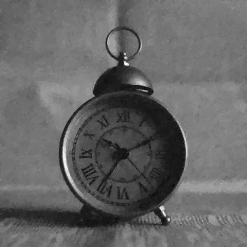 \(~\) \(~\) |
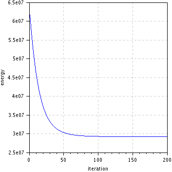 |
Several variants of the ROF model
Anisotropic total variation
Replacing the \(\ell^2\) norm of the gradient by a \(\ell^1\) norm into the definition of the total variation, we obtain the anisotropic total variation
\[ \forall u \in \RR^\Omega, \quad \TVani(u) = \| \nabla u \|_{1,1} := \sum_{(x,y) \in \Omega} \left| \nabla u (x,y) \right|_1 \;. \]
The primal problem
The anisotropic total variation variant of the ROF problem consists in replacing the \(\TV\) regularizer by \(\TVani\), the problem writes
\begin{equation} \label{eq:primal-rofani} % \widehat{u}_\text{MAP}^\text{ani} = \arg\, \min_{u \in \RR^\Omega} \tfrac{1}{2} \| u - u_0 \|_2^2 + \lambda \TVani(u) \;. % \end{equation}Primal-dual formulation
The dual formulation (see the proofs here) of \(\TVani\) is given by
\begin{equation*} % \forall u \in \RR^\Omega, \quad \TVani(u) = \max_{p \in \RRRR{\Omega}} \langle \nabla u , p \rangle \quad \text{subject to} \quad \|p\|_{\infty,\infty} \leq 1 \;, % \end{equation*}where \(\forall p \in \RRRR{\Omega}, \quad \| p \|_{\infty,\infty} = \max_{(x,y) \in \RR^\Omega} \left| p(x,y) \right|_\infty\) (noting \(|\cdot|_\infty\) the \(\ell^\infty\) norm over \(\RR^2\)). We get a primal-dual formulation of \eqref{eq:primal-rofani},
\begin{equation} \label{eq:primal-dual-rofani} % \widehat{u}_\text{MAP}^\text{ani} = \arg\, \min_{u \in \RR^\Omega} \, \max_{p \in \RRRR{\Omega}} \tfrac{1}{2} \| u - u_0 \|_2^2 + \langle \lambda \nabla u , p \rangle - \delta_\text{ani}(p)\;, % \end{equation}where \(\delta_\text{ani}\) denotes the indicator function of the closed unit ball for the norm \(\| \cdot \|_{\infty,\infty}\), that is
\begin{equation*} % \forall p \in\RRRR{\Omega}, \quad \delta_\text{ani} (p) = \left\{ \begin{array}{cl} 0 & \text{if } \| p \|_{\infty,\infty} \leq 1 \\ +\infty & \text{otherwise.} \end{array} \right. % \end{equation*}Chambolle-Pock algorithm. Replacing function \(\delta\) by \(\delta_\text{ani}\) into Algorithm 1, we obtain a resolvant algorithm for problem \eqref{eq:primal-dual-rofani}. Only the dual update is changed, we easily derive a closed-form formula.
Replacing \(\delta\) by \(\delta_\text{ani}\) into Equation \eqref{cp.dual} (the dual update of Algorithm 1), boils down to the pointwise operations
\[ \forall (i,j) \in \Omega, \quad p^{k+1}(i,j) = \left( p_x^{k+1}(i,j), p_y^{k+1}(i,j) \right) \]
where\(\quad p_x^{k+1}(i,j) = \mathcal{S} \left(p_x^k(i,j) + \sigma \lambda \nabla_x \bar{u}^k (i,j) \right)\), \(\quad p_y^{k+1}(i,j) = \mathcal{S} \left(p_y^k(i,j) + \sigma \lambda \nabla_y \bar{u}^k (i,j) \right)\),
and \(\mathcal{S}\) denotes the soft-thresholding operator which is defined by
\begin{equation*} % \forall a \in \RR, \quad \mathcal{S} (a) = \left\{ \begin{array}{ccc} -1 & \text{if} & a < -1 \\ a & \text{if} & -1 \leq a \leq 1 \\ 1 & \text{if} & 1 < a. \end{array} \right. % \end{equation*}Scilab implementation
//     Anisotropic TV restoration of Images Corrupted with Gaussian noise
//
// u0 = input image
// lambda = regularity parameter (TV weight)
// niter = number of iterations for the Chambolle-Pock algorithm
// u = restored image
// E = energy (E(i) = energy computed at iteration i)
//
function [u,E] = tvdenoise_anisotropic(u0,lambda,niter)
  //* initialization *//
  [ny,nx] = size(u0);
  E = zeros(niter,1);
  u = u0;
  ubar = u0;
  px = zeros(u0);
  py = zeros(u0);
  // precompute Chambolle & Pock algorithm step parameters
  tau = 0.99/(sqrt(8)*lambda);
  sigma = tau;
  theta = 1;
  //*************** main loop ***************//
  for i = 1:niter
    //* compute (Dx,Dy) = grad(ubar) *//
    [Dx,Dy] = grad(ubar);
    //* update p = (px,py) *//
    px  = px + sigma*lambda*Dx;
    px(px < -1) = -1;
    px(px >  1) =  1;
    py  = py + sigma*lambda*Dy;
    py(py < -1) = -1;
    py(py >  1) =  1;
    // * compute d = div(p) *//
    d = div(px,py);
    //* update u and ubar *//
    ubar = -theta * u;
    u = (u + tau*u0 + tau*lambda*d)/(1+tau);
    ubar = ubar + (1+theta)*u;
    //* compute energy of u *//
    [Dx,Dy] = grad(u);
    E(i) = sum(0.5*(u-u0).^2 + lambda*(abs(Dx) + abs(Dy)));
    printf("iteration %d : E = %.10g\n",i,E(i));
  end
  //************ end of main loop ************//
endfunction
Example
//* Open reference image & add noise *//
ref = readpgm('clock.pgm'); // change the path according to the location of the image on your disk.
sigma = 20; // set noise level (standard deviation)
u0 = ref + grand(ref,'nor',0,sigma); // add white Gaussian noise with zero-mean and standard deviation sigma;
imview(u0); // display input (noisy)

//* Run tvdenoise and tvdenoise_anisotropic algorithms *//
lambda = 15; // set regularity parameter
niter = 200; // choose a number of iterations for the Chambolle-Pock algorithm
u_iso = tvdenoise(u0,lambda,niter);
u_ani = tvdenoise_anisotropic(u0,lambda,niter);
imview(u_iso);
imview(u_ani);

//* zoom x3 (zero order) and crop outputs *//
z_iso = u_iso .*. ones(3,3); // zoom x3
z_ani = u_ani .*. ones(3,3); // zoom x3
imview(z_iso(281:633,301:653)); // display crop
imview(z_ani(281:633,301:653)); // display crop
| restored with isotropic \(\TV\) (\(\lambda=14\)) | restored with anisotropic \(\TV\) (\(\lambda=14\)) |
 \(~\) \(~\) |
 |
| nearest neighbor zoom \(\times 3\) | nearest neighbor zoom \(\times 3\) |
 \(~\) \(~\) |
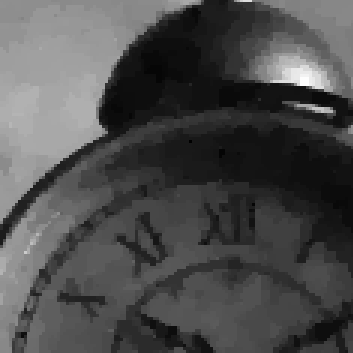 |
The anisotropic total variation variant of the ROF model leads to images with sharp horizontal and vertical edges.
Other variants. The use of the anisotropic total variation leads to interesting variants of the ROF model, such as [8,9].
The Huber total variation
The use of the discrete total variation as a regularizer for image processing applications has a main drawback, the so-called staircasing effect that is the creation of piecewise constant regions with artificial boundaries in the restored image. This undesirable effect has been rigorously identified and studied in [5,6,7], in particular it is proven (in a more general setting than total variation regularization) in [5] that the non-differentiability at zero of the total variation is responsible of the staircasing artifact.
In order to get rid of the staircasing artifact, we can to replace the \(\ell^2\) norm \(|\cdot|_2\) of the gradient by the Huber-function \(|\cdot|_\alpha\), defined as
\begin{equation} \label{eq:hubernorm} % \forall g \in \RR^2, \quad |g|_\alpha = \left\{ \begin{array}{cl} \frac{|g|_2^2}{2\alpha} & \text{if } |g|_2 \leq \alpha\;, \\ | g |_2 - \frac{\alpha}{2} & \text{otherwise}\;, \end{array} \right. % \end{equation}which is a smooth approximation of the $ℓ2$-norm (near \(0\) the \(\ell^2\) norm is being replaced by a quadratic \(\ell^2\) norm).
Given a parameter \(\alpha > 0\), the (discrete) Huber total variation with smoothness parameter \(\alpha\) writes
\[\forall u \in \RR^\Omega, \quad \HTValpha (u) = \sum_{(x,y) \in \Omega} \left| \nabla u (x,y) \right|_\alpha \;, \]
The primal problem
The Huber total variation variant of the ROF problem consists in replacing the \(\TV\) regularizer by \(\HTValpha\), the problem writes
\begin{equation} \label{eq:primal-huber-rof} % \widehat{u}_\text{MAP}^\text{Huber} = \arg\, \min_{u \in \RR^\Omega} \tfrac{1}{2} \| u - u_0 \|_2^2 + \lambda \HTValpha(u) \;. % \end{equation}Primal-dual formulation
The dual formulation (see the proofs here) of \(\HTValpha\) is given by
\begin{equation*} % \forall u \in \RR^\Omega, \quad \HTValpha(u) = \max_{p \in \RRRR{\Omega}} \langle \nabla u , p \rangle - \tfrac{\alpha}{2} \|p\|_2^2 \quad \text{subject to} \quad \|p\|_{\infty,2} \leq 1 \;, % \end{equation*}replacing accordingly the \(\HTValpha\) term in \eqref{eq:primal-rof}, we get a primal-dual reformulation of the problem
\begin{equation} \label{eq:primal-dual-huber-rof} % \widehat{u}_\text{MAP}^\text{Huber} = \arg\, \min_{u \in \RR^\Omega} \, \max_{p \in \RRRR{\Omega}} \tfrac{1}{2} \| u - u_0 \|_2^2 + \langle \lambda \nabla u , p \rangle - \delta(p) - \lambda \tfrac{\alpha}{2} \|p\|_2^2\;, % \end{equation}Chambolle-Pock algorithm. Replacing function \(\delta(p)\) by \(\delta(p)+\lambda \tfrac{\alpha}{2} \| p \|_2^2\) into Algorithm 1, leads to a resolvant algorithm for problem \eqref{eq:primal-dual-huber-rof}. Again, only the dual update is changed and we easily derive a closed-form formula.
Replacing \(\delta(p)\) by \(\delta(p)+\lambda \tfrac{\alpha}{2} \|p\|_2^2\) into Equation \eqref{cp.dual} (the dual update of Algorithm 1), boils down to the pointwise operations \[ % \forall (x,y) \in \Omega, \quad p^{k+1}(x,y) = \frac{\left(p^k(x,y) + \sigma \lambda \nabla \bar{u}^k(x,y) \right) / \nu }{\max { \left( 1 , \left|\, \left( p^k(x,y) + \sigma \lambda \nabla \bar{u}^k(x,y) \right) / \nu \,\right|_2 \right) }} \;, % \] where \(\nu = 1+\sigma \alpha \lambda\).
Scilab implementation
//     Huber-TV restoration of Images Corrupted with Gaussian noise
//
// u0 = input image
// alpha = Huber smoothness parameter
// lambda = regularity parameter (TV weight)
// niter = number of iterations for the Chambolle-Pock algorithm
// u = restored image
// E = energy (E(i) = energy computed at iteration i)
//
function [u,E] = tvdenoise_huber(u0,alpha,lambda,niter)
  //* initialization *//
  [ny,nx] = size(u0);
  E = zeros(niter,1);
  u = u0;
  ubar = u0;
  px = zeros(u0);
  py = zeros(u0);
  // precompute Chambolle & Pock algorithm step parameters
  tau = 0.99/(sqrt(8)*lambda);
  sigma = tau;
  theta = 1;
  nu = 1+sigma*alpha*lambda;
  //*************** main loop ***************//
  for i = 1:niter
    //* compute (Dx,Dy) = grad(ubar) *//
    [Dx,Dy] = grad(ubar);
    //* update p = (px,py) *//
    px  = (px + sigma*lambda*Dx)/nu;
    py  = (py + sigma*lambda*Dy)/nu;
    nrm = px.*px + py.*py;
    id = nrm > 1; nrm = sqrt(nrm(id));
    px(id) = px(id) ./ nrm;
    py(id) = py(id) ./ nrm;
    // * compute d = div(p) *//
    d = div(px,py);
    //* update u and ubar *//
    ubar = -theta * u;
    u = (u + tau*u0 + tau*lambda*d)/(1+tau);
    ubar = ubar + (1+theta)*u;
    //* compute energy of u *//
    [Dx,Dy] = grad(u);
    nrm = Dx.^2 + Dy.^2;
    id = (nrm <= alpha^2);
    htv = 0.5/alpha*sum(nrm(id)) + sum(sqrt(nrm(~id))-alpha/2);
    E(i) = 0.5*sum((u-u0).^2) + lambda*htv;
    printf("iteration %d : E = %.10g\n",i,E(i));
  end
  //************ end of main loop ************//
endfunction
Example
//* Open reference image & add noise *//
ref = readpgm('clock.pgm'); // change the path according to the location of the image on your disk.
sigma = 20; // set noise level (standard deviation)
u0 = ref + grand(ref,'nor',0,sigma); // add white Gaussian noise with zero-mean and standard deviation sigma;
imview(u0); // display input (noisy)

//* Run tvdenoise and tvdenoise_huber algorithms *//
lambda = 15; // set regularity parameter
niter = 200; // choose a number of iterations for the Chambolle-Pock algorithm
alpha = 7;   // set the Huber smoothness parameter
u_iso = tvdenoise(u0,lambda,niter);
u_hub = tvdenoise_huber(u0,alpha,lambda,niter);
imview(u_iso);
imview(u_hub);

//* zoom x3 (zero order) and crop outputs *//
z_iso = u_iso .*. ones(3,3); // zoom x3
z_hub = u_hub .*. ones(3,3); // zoom x3
imview(z_iso(281:633,301:653)); // display crop
imview(z_hub(281:633,301:653)); // display crop
| restored with isotropic \(\TV\) (\(\lambda=14\)) | restored with \(\HTValpha\) (\(\lambda=14\), \(\alpha=7\)) |
 \(~\) \(~\) |
 |
| nearest neighbor zoom \(\times 3\) | nearest neighbor zoom \(\times 3\) |
 \(~\) \(~\) |
 |
The Huber variant of the ROF model does not introduce any numerical nor mathematical difficulty and leads to more natural images free of staircasing artifact, although a bit less sharp than those obtained with the classical ROF model.
References
- Rudin, L. I., Osher, S., and Fatemi, E.: ``Nonlinear total variation based noise removal algorithms'', Physica D 60(1), pp. 259–268, 1992.
- Ekeland, I., and Témam, R.: ``Convex analysis and variational problems'', volume 28 of Classics in Applied Mathematics. Society for Industrial and Applied Mathematics (SIAM), Philadelphia, PA, english edition, 1999. Translated from the French.
- Chambolle, A., Pock, T.: ``A first-order primal-dual algorithm for convex problems with applications to imaging'', Journal of Mathematical Imaging and Vision, vol. 40, pp. 120–145, 2011.
- Chambolle, A., Caselles, V., Cremers, D., Novaga, M., and Pock, T.: `` An introduction to total variation for image analysis'', Theoretical foundations and numerical methods for sparse recovery, 9, 263–340, 2010.
- Nikolova, M.: ``Local Strong Homogeneity of a Regularized Estimator'', SIAM Journal on Applied Mathematics, vol. 61, pp. 633–658, 2000.
- Chan, T. F., Marquina, A., and Mulet, P.: ``Higher Order Total Variation-Based Image Restoration'', SIAM Journal on Scientific Computing, vol. 22, pp. 503–516, 2000.
- Ring, W.: ``Structural Properties of Solutions to Total Variation Regularization Problems'', M2AN, Modélisation Mathématique et Analyse Numérique, vol. 34, pp. 799–810, 2000.
- Louchet, C., and Moisan, L.: ``Total variation denoising using iterated conditional expectation'', In proceedings of the European Signal Processing Conference (Eusipco), 2014.
- Abergel, R., Louchet, C., Moisan, L., and Zeng, T.: ``Total Variation Restoration of Images Corrupted by Poisson Noise with Iterated Conditional Expectations'', In Scale Space and Variational Methods in Computer Vision, pp. 178-190, Springer International Publishing, 2015.