Color transfer between images
For the following exercices, you need either Matlab or Scilab. Please read the introduction page to download the images used in the exercices and to learn how to read and display images with Scilab.
The goal of the following exercices is to test several ways to transfer color palettes between two images \(u\) and \(v\) of the same size.
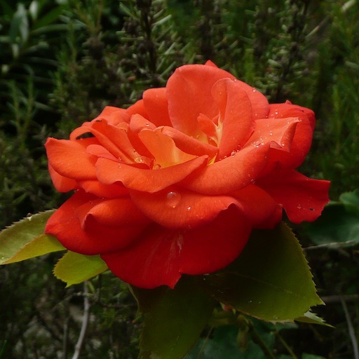
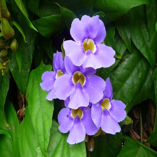
u = read_bmp_bg('im/flower1.bmp');  // use imread with Matlab
v = read_bmp_bg('im/flower2.bmp');
[nr,nc,nch] = size(u);
ccview(u);                          // imshow(u,[]) with Matlab
ccview(v);
Sommaire
1 Separable affine transfer
Beware of the fact that the function mean is different under Matlab and Scilab. It computes the total mean of a matrix under Scilab, whereas it returns the mean value along the first array dimension of the matrix under Matlab.
Write a function affine_transfer which apply an affine transform to \(u\) such that it has the same mean and the same standard deviation as \(v\) on each channel.
function w = affine_transfer(u,v)
  for i = 1:3
      INSERT YOUR CODE
  end
endfunction
Display and comment the result.
w = affine_transfer(u,v);
w = min(max(w,0),255);
ccview(w);                       // Matlab : imshow
2 Separable specification
Another solution consists in applying histogram specifications separately on each channel of the images \(u\) and \(v\).
function w = specification_channels(u,v)
  for i = 1:3
    uch = u(:,:,i);
    vch = v(:,:,i);
    INSERT YOUR CODE
  end
endfunction
Display and comment the result.
w = specification_channels(u,v);
w = min(max(w,0),255);
ccview(w);                     // imshow
3 Affine transfer in a color space with decorrelated channels
The RGB color space is not very well suited for these operations since the channels R, G and B are strongly correlated. Instead, we can first convert the RGB images to another color space with less correlation between channels. For instance, we can use a color opponent space with an achromatic channel and two chromatic channels representing an approximate red-green opponency and yellow- blue opponency :
$$ O_1 = \frac 1 {\sqrt{2}} (R-G),\; O_2 = \frac 1 {\sqrt{6}} (R+G-2B),\; O_3 = \frac 1 {\sqrt{3}} (R+G+B)$$Apply the separable color transfers (affine and specification) to \(u\) and \(v\) in this opponent color space. Is the result more satisfying ?
O = [1/sqrt(3), 1/sqrt(3), 1/sqrt(3) ; 1/sqrt(2) -1/sqrt(2) 0; 1/sqrt(6) 1/sqrt(6) -2/sqrt(6)];
u_opp = matrix(matrix(u,nr*nc,3)*O',nr,nc,3);      // Matlab : replace 'matrix'  by 'reshape'
v_opp = matrix(matrix(v,nr*nc,3)*O',nr,nc,3);
//w_opp = affine_transfer(u_opp,v_opp);
w_opp = specification_channels(u_opp,v_opp);
w_opp = matrix(matrix(w_opp,nr*nc,3)*inv(O)',nr,nc,3);
w_opp = min(max(w_opp,0),255);
ccview(w_opp);                                     // Matlab  : imshow
As adviced in the works of Reinhard et al., these separable transformations can also be applied in the \(L\alpha\beta\) color space (see the following pdf).
LMS = [0.3811 0.5783 0.0402 ; 0.1967 0.7244 0.0782 ; 0.0241 0.1288 0.8444];
u_lms = log10(0.1+matrix(matrix(u,nr*nc,3)*LMS',nr,nc,3));
v_lms = log10(0.1+matrix(matrix(v,nr*nc,3)*LMS',nr,nc,3));
u_lab = matrix(matrix(u_lms,nr*nc,3)*O',nr,nc,3);
v_lab = matrix(matrix(v_lms,nr*nc,3)*O',nr,nc,3);
w_lab = affine_transfer(u_lab,v_lab);
//w_lab = specification_channels(u_lab,v_lab);
w_lms = matrix(matrix(w_lab,nr*nc,3)*inv(O)',nr,nc,3);
w_lms = matrix(matrix(exp(w_lms*log(10))-0.1,nr*nc,3)*inv(LMS)',nr,nc,3);
Display and comment the results.
w_lms = min(max(w_lms,0),255);
ccview(w_lms);
4 Sliced optimal transport
In order to transport the full color distribution of \(u\) on the one of \(v\), we propose to write these distributions as 3D point clouds \begin{equation} X = \begin{pmatrix} X_1 \\ \vdots\\ X_n \end{pmatrix}, \;\;\text{ and }\;\; Y = \begin{pmatrix} Y_1 \\ \vdots\\ Y_n \end{pmatrix}, \end{equation} with \(n\) the number of pixels in \(u\) and \(v\), \(X_i\) the color \((R_i,G_i,B_i)\) of the \(i\)-th pixel in \(u\) and \(Y_i\) the color of the \(i\)-th pixel in \(v\) (\(X\) and \(Y\) are \(n\times 3\) matrices). We look for the permutation \(\sigma\) of \(\{1,\dots, n\}\) which minimizes the quantity \begin{equation} \label{eq:transport_appariement} \sum_{i=1}^n \|X_i - Y_{\sigma(i)}\|^2_2. \end{equation} The assignment \(\sigma\) defines a mapping between the set of colors \(\{X_i\}_{i=1,\dots n}\) and the set of colors \(\{Y_j\}_{j=1,\dots n}\).
4.1 1D Transport
In one dimension, the assignment \(\sigma\) which minimizes the previous cost is the one which preserves the ordering of the points. More precisely, if \(\sigma_X\) and \(\sigma_Y\) are the permutations such that $$X_{\sigma_X(1)} \leq X_{\sigma_X(2)} \leq \dots \leq X_{\sigma_X(n)},$$ $$Y_{\sigma_Y(1)} \leq Y_{\sigma_Y(2)} \leq \dots \leq Y_{\sigma_Y(n)},$$ then \(\sigma = \sigma_Y \circ \sigma_X^{-1}\) minimizes the previous cost.
The following function transport1D takes two 1D point clouds \(X\) and \(Y\) and return the permutations \(\sigma_X\) and \(\sigma_Y\).
function [sX,sY] = transport1D(X,Y)
    [Xs,sX] = gsort(X,'g','i');   // We have Xs = X(sX)  // Matlab : sort(X)
    [Ys,sY] = gsort(Y,'g','i');
endfunction
4.2 Sliced 3D Transport
Finding the solution of the assignment problem in more than one dimension is computationnaly demanding. Instead of computing the explicit solution, we make use of a stochastic gradient descent algorithm which computes the solution of a sliced approximation of the oprimal transport problem over 1D distributions (see the following paper).
The algorithm starts from the point cloud \(Z=X\). At each iteration, it picks a random orthonormal basis of \(\mathbb{R}^3\), denoted by \((u_1,u_2,u_3)\), and for each \(k=1,\dots 3\) it computes the gradient step
$$ Z_{\sigma_Z} = Z_{\sigma_Z} + \varepsilon ( (Y,u_k)_{\sigma_Y} - (Z,u_k)_{\sigma_Z} ) u_k,$$where \((\;,\;)\) is the scalar product in \(\mathbb{R}^3\), \(\sigma_Y\) and \(\sigma_Z\) are the permutations that order the one-dimensionnal projected point clouds \(\{(Y_j,u_k)\}_{j=1\dots n}\) and \(\{(Z_j,u_k)\}_{j=1\dots n}\).
function Z=transport3D(X,Y,N,e)  // X, Y and Z are  n x 3 matrices
  Z = X;
  for k=1:N

    // orthogonal basis, uniform distribution on the sphere
    u = rand(3,3,'normal');
    q = qr(u);

    // projection
    for j=1:3
      Zt = Z*q(:,j);
      Yt = Y*q(:,j);
     INSERT YOUR CODE
    end
  end
endfunction
Test the previous code with random 3D point clouds.
X = rand(20,3);
Y = rand(20,3);
Z = transport3D(X,Y,5000,0.01);
param3d1(X(:,1),X(:,2),list(X(:,3),-1));  // points of X are represented as +
param3d1(Y(:,1),Y(:,2),list(Y(:,3),-2));  // points of Y are represented as x
param3d1(Z(:,1),Z(:,2),list(Z(:,3),-3));   // points of Y are represented as o
Visualize the displacement of the point cloud \(X\) toward \(Y\).
Z=X;
figure;param3d1(X(:,1),X(:,2),list(X(:,3),-1));
param3d1(Y(:,1),Y(:,2),list(Y(:,3),-2));
param3d1(Z(:,1),Z(:,2),list(Z(:,3),-3));
f=gca(); // handle current graphic
sleep(1000); // pause
for i=1:60
   Z = transport3D(Z,Y,100,0.01);
   f.children(3).data=Z; // modify the coordinates of the third point cloud
   sleep(100);
end
4.3 Use for color transfer
First subsample images to reduce the number of points.
u = u(1:4:nr,1:4:nc,:);
v = v(1:4:nr,1:4:nc,:);
[nr,nc,nch] = size(u);
Create the color point clouds from the subsampled color images,
X = matrix(u,nr*nc,3);
Y = matrix(v,nr*nc,3);
Then apply the previous sliced optimal transport algorithm to compute the optimal assignment between the point clouds and display the resulting image.
Z = transport3D(X,Y,1000,0.01);
w = matrix(Z,nr,nc,3);
w = min(max(w,0),255);
ccview(w);
5 Barycenter and midway
Knowing the optimal (or an approximation) assignment between the point clouds \(X\) and \(Y\), you can compute barycenters between these discrete distributions. Use the previous results to compute the midway color distribution between \(u\) and \(v\) and the corresponding midway images.
6 Regularization
A common drawback of classical methods aiming at color and contrast modifications is the revealing of artefacts (JPEG blocs, color inconsistancies, noise enhancement) or the attenuation of details and textures (see for instance the following web page). Let \(u\) be an image and \(g(u)\) the same image after color or contrast modification, we write \(\mathcal{M}(u) = g(u) - u\). All artefacts observable in \(g(u)\) can be seen as irregularities in the map \(\mathcal{M}(u)\). In order to reduce these artefacts, we propose to filter this difference map thanks to an operator \(Y_u\) and to reconstruct the image :
$$T(g(u)) = u + Y_u(g(u)-u).$$Let us begin with a very simple averaging filter for \(Y_u\).
K = ones(4,4); K = K/sum(K);
for i=1:3
  wreg(:,:,i) = INSERT YOUR CODE HERE
end
Display the result
wreg = min(max(wreg,0),255);
ccview(wreg);
A more interesting result can be obtained by filtering the difference map \(\mathcal{M}(u)\) in order to follow the regularity of \(u\). To this aim, we define the operator \(Y_u\), a weighted average with weights depending on the similarity of pixels in the original image \(u\). The effect of this operator on an image \(u_0\) is defined as $$Y_u (u_0)(x) = \frac{1}{c(x)} \sum_{y \in \mathcal{V}(x)} u_0(y) w_u (x,y),$$ with \(\mathcal{V}(x)\) a square neighborhood of \(x\) and \(c(x)\) the normalization constant \(c(x) = \sum_{y \in \mathcal{V}(x)} w_u (x,y)\). The weights \(w_u (x, y)\) are defined as $$w_u (x, y) = e^{-\| u(x)−u(y) \|^2 / h^2 },$$ with \(\|.\|\) the Euclidean distance in \(\mathbb{R}^3\). and \(\mathcal{V}(x)\) a square neighborhood of \(x\). Observe that if we apply \(Y_u\) to the image \(u\), we obtain the Yaroslavsky filter.
- Write a function
crossed_filterwhich computes the previously described filter.
function b=crossed_filter(u,u0,f,sigma)
    // the goal is to regularize u0 following the regularity of u
    [nrow,ncol]=size(u);

    for i=1:nrow
        for j=1:ncol
         // Extract a neighborhood of (i,j)
         iMin = max(i-f,1);
         iMax = min(i+f,nrow);
         jMin = max(j-f,1);
         jMax = min(j+f,ncol);
         v = u(iMin:iMax,jMin:jMax,:);
         v0 = u0(iMin:iMax,jMin:jMax,:);
         // Compute gaussian weights
         INSERT YOUR CODE
        // Compute the filtered image at (i,j)
         INSERT YOUR CODE
        end
    end
endfunction
Apply the previous filter to \(\mathcal{M}(u)\) and display the result \(T(g(u))\). In order to remove the aforementioned artefacts, you can iterate the filter.