Minimizing the total variation under affine constraints

General formulation
Primal-dual reformulation
Computational procedure
Applications
Elements of comparison with the inverse problem framework
The Huber total variation variant
References

General formulation

We are interested in computing an image having the smallest total variation among the images $u_0$ satisfying an affine constraint of kind $Au = u_0$ for a given linear operator $A: \RR^\Omega \mapsto \RR^\omega$ ($\Omega$ and $\omega$ being two rectangular subsets of $\ZZ^2$) and a given $u_0 \in \RR^\omega$. The problem consists in computing $\widehat{u}_\text{constr}$ such as

\begin{equation} \label{eq:primal-tvconstr} % \widehat{u}_\text{constr} = \arg \, \min_{u \in \RR^\Omega} \TV(u) \quad \text{subject to} \quad Au = u_0\;. % \end{equation}

Note the similarity with the inverse problem (see here the page dedicated to inverse problems) which writes (for a given $\lambda > 0$),

\begin{equation} \label{eq:primal-inverse} % \widehat{u}_\text{inverse} = \arg \, \min \tfrac{1}{2} \|Au - u_0\|_2^2 + \lambda \TV(u) \;. % \end{equation}

The inverse problem \eqref{eq:primal-inverse} can be seen as a reformulation of problem \eqref{eq:primal-tvconstr} where the constraint $Au = u_0$ has been relaxed. Indeed any image $\widehat{u}_\text{constr}$ satisfying \eqref{eq:primal-tvconstr} must verify exactly the constraint $A \widehat{u}_\text{constr} = u_0$, while an image $\widehat{u}_\text{inverse}$ satisfying \eqref{eq:primal-inverse} is such as $A \widehat{u}_\text{inverse} \approx u_0$ since it realizes a compromise between minimizing $\|Au - u_0\|_2^2$ and $\TV(u)$ (in fact the smaller $\lambda$ is, the stronger is the data fidelity term $\tfrac{1}{2}\|Au -u_0\|_2^2$ compared to the regularity term $\lambda \TV(u)$ and thus, the closer to each other $A \widehat{u}_\text{inverse}$ and $u_0$ are).

In practice when the given data $u_0$ is corrupted with noise, working with \eqref{eq:primal-inverse} makes sense because it allows $Au \neq u_0$ (here $u$ denotes the restored image). However when the amount of noise is low, problem \eqref{eq:primal-tvconstr} becomes interesting since it avoids to the user the setting of the parameter $\lambda$.

Of course problems \eqref{eq:primal-tvconstr} and \eqref{eq:primal-inverse} become equivalent when $\lambda > 0$ is choosen small enough (in the sense that the solutions of those two problems can be set arbitrarily close to each other), however we will see on several examples that the Chambolle-Pock algorithm used to numerically compute the solution of the inverse problem (see here the algorithm) shows very slow convergence when $\lambda$ is small whereas it will not be the case when applying the Chambolle-Pock algorithm to the constrained problem \eqref{eq:primal-tvconstr}.

Primal-dual reformulation

Recall the dual formulation of the discrete total variation (see here the page dedicated to the discrete total variation)

$$ \TV(u) = \max_{p \in \RRRR{\Omega}} \langle \nabla u , p \rangle \quad \text{subject to} \quad \|p\|_{\infty,2} \leq 1 \;, $$

where $\|p\|_{\infty,2} = \max_{(x,y) \in \RR^\Omega} \|p(x,y)\|_2$.

Noting $\delta$ the indicator function of the closed unit ball of the norm $\|\cdot\|_{\infty,2}$, that is

\begin{equation*} \forall p \in \RRRR{\Omega}, \quad \delta(p) = \left\{ \begin{array}{cl} 0 & \text{if } \|p\|_{\infty,2} \leq 1 \\ +\infty & \text{otherwise,} \end{array} \right. \end{equation*}

and replacing the $\TV$ term by its dual formulation into equation \eqref{eq:primal-tvconstr} we obtain a primal-dual (saddle-point) reformulation of the problem,

\begin{equation} \label{eq:primal-dual-tvconstr-interm} % \widehat{u}_\text{constr} = \arg \, \min_{u \in \RR^\Omega} \, \max_{p \in \RRRR{\Omega}} \langle \nabla u , p \rangle - \delta(p) \quad \text{subject to} \quad Au = u_0 \;. % \end{equation}

Noting $\delta_{A^{-1}u_0}$ denotes the indicator function of the convex set $A^{-1}u_0 := \left\{ u \in \RR^\Omega, ~ Au = u_0 \right\}$,

\begin{equation*} \forall u \in \RR^\Omega, \quad \delta_{A^{-1}u_0}(u) = \left\{ \begin{array}{cl} 0 & \text{if } Au = u_0 \\ +\infty & \text{otherwise,} \end{array} \right. \end{equation*}

the problem \eqref{eq:primal-dual-tvconstr-interm} can be reformulated as

\begin{equation} \label{eq:primal-dual-tvconstr} % \widehat{u}_\text{constr} = \arg \, \min_{u \in \RR^\Omega} \, \max_{p \in \RRRR{\Omega}} \delta_{A^{-1}u_0}(u) + \langle \nabla u , p \rangle - \delta(p) \;, % \end{equation}

and this problem can be numerically solved thanks the Chambolle and Pock algorithm [3].

Computational procedure

The Chambolle and Pock algorithm

A solution of problem \eqref{eq:primal-dual-tvconstr} can be numerically computed using the algorithm of Chambolle-Pock [3], which is designed to solve the generic saddle-point problem

\begin{equation} \label{eq:cp.primal-dual} \arg\,\min_{x \in X}\max_{y \in Y} ~ G(x) + \langle Kx , y \rangle - F^\star(y) \;. \end{equation}

The algorithm is briefly presented on this page.

Taking $X=\RR^\Omega$, $Y=\RRRR{\Omega}$, $F^\star = \delta$, $G = \delta_{A^{-1}u_0}$ and $K = \nabla$ into problem \eqref{eq:cp.primal-dual} allows to recover problem \eqref{eq:primal-dual-tvconstr}.

We note $\divergence = -\nabla^*$ the opposite of the adjoint of the operator $\nabla$ (in analogy with the continuous setting), the Chambolle and Pock algorithm applied to problem \eqref{eq:primal-dual-tvconstr} boils down to Algorithm 1.

Chambolle-Pock resolvant algorithm for problem \eqref{eq:primal-dual-tvconstr}.

Initialization: Choose $\tau, \sigma > 0$, $\theta \in [0,1]$, $u^0 \in \RR^\Omega$, $p^0 \in \RRRR{\Omega}$ and set $\bar{u}^0 = u^0$.

Iterations ($k \geq 0$): Update $u^k,p^k$ and $\bar{u}^k$ as follows

\begin{eqnarray} p^{k+1} &=& \arg\,\min\limits_{\substack{p \in \RRRR{\Omega} }} ~ \tfrac{1}{2\sigma} \left\|p-(p^k+\sigma \nabla \bar{u}^k)\right\|_2^2 + \delta(p) \label{cp.dual} \\ u^{k+1} &=& \arg\,\min\limits_{\substack{u \in \RR^\Omega}} ~ \tfrac{1}{2\tau} \left\|u-\left(u^k +\tau \divergence p^{k+1} \right)\right\|_2^2 + \delta_{A^{-1}u_0}(u) \label{cp.primal} \\ \bar{u}^{k+1} &=& u^{k+1} + \theta \left(u^{k+1}-u^{k}\right) \nonumber \end{eqnarray}

$~$

The dual update (Equation \eqref{cp.dual}) can be computed in closed-form, the primal update (Equation \eqref{cp.primal}) consists in a $\ell^2$ projection over the convex set $A^{-1}u_0$, which may be non-trivial according to the choice of $A$.

The dual update \eqref{cp.dual} boils down to the pointwise operations $$ % \forall (x,y) \in \Omega, \quad p^{k+1}(x,y) = \frac{p^k(x,y) + \sigma \nabla \bar{u}^k(x,y) }{\max { \left( 1 , \left|\, p^k(x,y) + \sigma \nabla \bar{u}^k(x,y) \,\right|_2 \right) }} \;, % $$ and the primal update \eqref{cp.primal} is $$ u^{k+1} = \pi_{A^{-1}u_0} \left( u^k(x,y) + \tau \divergence p^{k+1} \right) \;, $$ where $\pi_{A^{-1}u_0}$ denotes the $\ell^2$ projection over the convex set $A^{-1}u_0 = \left\{ u \in \RR^\Omega, ~ Au = u_0 \right\}$.

Notice that the convergence of Algorithm 1 toward a solution of problem \eqref{eq:primal-dual-tvconstr} is ensured when $\theta = 1$ and $\tau \sigma {|||K|||}^2 < 1$. Here we have ${|||K|||}^2 = \lambda^2 {|||\nabla|||}^2$, wich depends on the choice of the discretization scheme used for $\nabla$.

Discretization schemes

Let $n_x$ and $n_y$ denote the width and height of the initial (noisy) image $u_0$, we note $\Omega = \left\{ 1, \dots , n_x \right\} \times \left\{ 1, \dots , n_y \right\}$ the discrete domain of $u_0$. We propose here to use the following finite difference scheme for the gradient operator

$$ \forall u \in \RR^\Omega, \quad \forall (i,j) \in \Omega, \quad \nabla u (i,j) = \left( \nabla_x u (i,j), \nabla_y u (i,j) \right)\;, $$

where

\begin{equation*} % \nabla_x u (i,j) = \left\{ \begin{array}{cl} u(i+1,j) - u(i,j) & \text{if } i < n_x \\ 0 & \text{if } i=n_x \end{array} \right. % \quad % \nabla_y u (i,j) = \left\{ \begin{array}{cl} u(i,j+1) - u(i,j) & \text{if } j < n_y \\ 0 & \text{if } j = n_y \end{array} \right. % \end{equation*}

This operator is easily implementable in Scilab langage,

function [Dx,Dy] = grad(u)
  [ny,nx] = size(u);
  Dx = u(:,[2:nx,nx]) - u;
  Dy = u([2:ny,ny],:) - u;
endfunction

and we can prove that the corresponding divergence operator (the opposite of the adjoint of $\nabla$) is given by

$$ \forall p = (p_x,p_y) \in \RRRR{\Omega}, \quad \forall (i,j) \in \Omega, \quad \divergence{(p)}(i,j) = \text{div}_x (p_x)(i,j) + \text{div}_y (p_y)(i,j) \;, $$

where

\begin{equation*} % \text{div}_x (p_x)(i,j) = \left\{ \begin{array}{cl} p_x(i,j)-p_x(i-1,j) & \text{if } 1 < i < n_x \\ p_x(i,j) & \text{if } i = 1 \\ -p_x(i-1,j) & \text{if } i = n_x \\ \end{array} \right. % \quad % \text{div}_y (p_y)(i,j) = \left\{ \begin{array}{cl} p_y(i,j)-p_y(i,j-1) & \text{if } 1 < j < n_y \\ p_y(i,j) & \text{if } j = 1 \\ -p_y(i,j-1) & \text{if } j = n_y \\ \end{array} \right. \end{equation*}

This operator is also easily implementable in Scilab langage.

function d = div(px,py) // compute d = div(p) where p = (px,py) and size(px) == size(py)
  [ny,nx] = size(px);
  div_x      =  px - px(:,[1,1:(nx-1)]);
  div_x(:,1) =  px(:,1);
  div_x(:,nx) = -px(:,nx-1);
  div_y      =  py - py([1,1:(ny-1)],:);
  div_y(1,:) =  py(1,:);
  div_y(ny,:) = -py(ny-1,:);
  d = div_x + div_y;
endfunction

Scilab implementation of the Chambolle Pock algorithm

With the choice of discretization scheme described in the previous section, we can show that the induced $\ell^2$ norm of the operator $\nabla$ is less than $\sqrt{8}$ (that is ${|||\nabla|||} \leq \sqrt{8}$), therefore taking $\tau = \sigma = \tfrac{0.99}{\sqrt{8}}$ into Algorithm 1 ensures that $\tau \sigma \, {|||K|||}^2 < 1$ (which, in addition to the setting $\theta=1$ is sufficient to ensure the convergence of the algorithm toward a solution of problem \eqref{eq:primal-dual-tvconstr}).

We propose below a Scilab implementation of Algorithm 1 that can be used to compute a solution of \eqref{eq:primal-tvconstr} once the projection $\pi_{A^{-1}u_0}$ has been set into Scilab memory

//* define the l2 projection of u over the set A^{-1}u0 = {w, Aw = u0} *//
function v = proj_constraint(u,u0)
  //* enter your code here *//
  ...
endfunction

Once the setting is done (accordingly to your choice for $A$), you can use the following implementation of Algorithm 1 to compute a solution of the constrained problem \eqref{eq:primal-tvconstr} with the Chambolle and Pock algorithm.

// u : denoised image,
// E : energy of u computed at each iteration
// u0 : input data (with domain omega)
// nx,ny : width and height of Omega (full domain)
// niter : number of iterations
function [u,E] = tvconstrained(u0,nx,ny,niter)
  //* initialization *//
  E = zeros(niter,1);
  u = zeros(ny,nx);
  ubar = u;
  px = zeros(ny,nx);
  py = zeros(ny,nx);
  // precompute Chambolle & Pock algorithm step parameters
  tau = 0.99/sqrt(8);
  sigma = tau;
  theta = 1;
  //*************** main loop ***************//
  for i = 1:niter
    //* compute (Dx,Dy) = grad(ubar) *//
    [Dx,Dy] = grad(ubar);
    //* update p = (px,py) *//
    px  = px + sigma*Dx;
    py  = py + sigma*Dy;
    nrm = px.*px + py.*py;
    id = nrm > 1; nrm = sqrt(nrm(id));
    px(id) = px(id) ./ nrm;
    py(id) = py(id) ./ nrm;
    // * compute d = div(p) *//
    d = div(px,py);
    //* update u and ubar *//
    ubar = -theta * u;
    u = proj_constraint(u + tau*d,u0);
    ubar = ubar + (1+theta)*u;
    //* compute energy of u *//
    [Dx,Dy] = grad(u);
    E(i) = sum(sqrt(Dx.^2 + Dy.^2));
    printf("iteration %d : E = %.10g\n",i,E(i));
  end
  //************ end of main loop ************//
endfunction

Applications

Basic tools for image manipulation in Scilab

We first propose some very basic tools dedicated to image manipulation in Scilab (opening, visualization).

Image viewer

function imview(u)
  [height,width] = size(u);
  fg = figure();
  set(fg,"axes_size",[width,height],"infobar_visible","on","menubar_visible","on","toolbar_visible","off","auto_resize","off","color_map",graycolormap(256));
  set(fg.children,"margins",zeros(1,4));
  Matplot(255/(%eps+max(u)-min(u)) * (u-min(u)),"010",[1,1,width,height]);
endfunction

Image opening (format PMG)

// open a PGM RAW image (8 bits)
// usage: u = readpgm('lena.pgm');
function image=readpgm(filename)
  //* local function *//
  function l=getline(u)
    h=[]
    while %t
      c=mget(1,'uc',u)
      if c==10 then break, end
      h=[h c]
    end
    l=ascii(h)
  endfunction
  //* main *//
  [u,err]=mopen(filename,'rb')
  if err<>0 then error('Impossible to open file '+filename), end
  if getline(u)~='P5' error('Unrecognized format'), end
  z=getline(u), while part(z,1)=='#', z=getline(u), end
  execstr('n=['+z+']')
  getline(u)
  image=matrix(mget(n(1)*n(2),'uc',u),n)'
  mclose(u)
endfunction

Inpainting (or disocclusion)

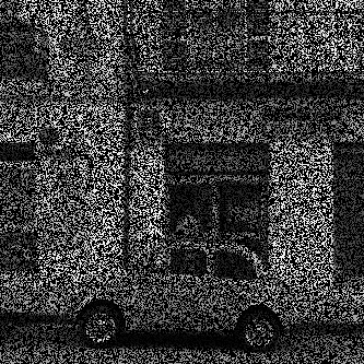
In this application, we will assume that some parts of the original image are missing, more precisely we suppose that the values of the pixels are known only on a given subset $\omega$ of $\Omega$, $u_0 \in \RR^\omega$ is non other than the restriction of the original image to the subset $\omega$, and the corresponding operator $A$ is simply the operator of restriction to $\omega$

$$\forall u \in \RR^\Omega, \quad Au = u_{|\omega} \in \RR^\omega \;.$$

The $\ell^2$ projection over $A^{-1} u_0$ is given by

\begin{equation*} % \forall u \in \RR^\Omega, \quad \forall (x,y) \in \Omega, \quad \pi_{A^{-1}u_0}(u) = \left\{ \begin{array}{cl} u_0(x,y) & \text{if } (x,y) \in \omega \\ u(x,y) & \text{otherwise.} \end{array} \right. % \end{equation*}

The reference image fiat.pgm used in this section is downloadable in PGM RAW format here (licence: CC0 public domain, source). We will define $\omega$ as the realization of a random subset of $\Omega$.

//* load the reference image *//
ref = readpgm('fiat.pgm'); // change the path according to the location of the image on your disk.
imview(ref); // display reference image

//* compute the subset omega of Omega *//
omega = (rand(ref) > 0.6); // aroud 60 % of the pixels are unknown
u0 = ref(omega); // restriction of the reference to omega
imview(ref.*double(omega)); // display input data (unknown pixels are set to zero for the display)

reference	observation (black = missing pixels)
$~$

The $\ell^2$ projection over $A^{-1}u_0$ is easily implementable in Scilab

function v = proj_constraint(u,u0)
  v = u;
  v(omega) = u0;
endfunction

We can now run our algorithm tvconstrained to numerically solve Problem \eqref{eq:primal-tvconstr}.

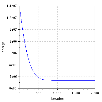
niter = 2000;
[ny,nx] = size(ref);
[u,E] = tvconstrained(u0,nx,ny,niter);
imview(u); // display restored image
figure(); plot(1:niter,E); // plot energy evolution
xlabel("iteration"); ylabel("energy");
title("Energy decrease");

observation (black = missing pixels)	restored
$~$

energy decrease

Zooming

Let us consider now the zooming operator (already studied in the inverse problem framework). For such application, the operator A is oftenly assumed to be a blurring kernel followed by a subsampling procedure (see [6,3]).

We consider two discrete domains, a (small) domain $\omega = \left[ 0, M \right) \times \left[ 0, N \right) \cap \ZZ^2$, and a (bigger) domain $\Omega = \left[ 0, z M \right) \times \left[ 0, z N \right) \cap \ZZ^2$, where $z$ denotes a given positive integer (zoom factor). We set $\omega_A = \left[0,z\right) \times \left[0, z\right) \cap \ZZ^2$ and define $A: \RR^\Omega \mapsto \RR^\omega$ by

\begin{equation} \label{eq:captor_integration} \forall u \in \RR^\Omega, \quad \forall (x,y) \in \omega, \quad Au(x,y) = \frac{1}{z^2} \sum_{(a,b) \in \omega_A} u(zx+a, zy+b)\;. \end{equation}

Remark that $Au$ is nothing more than a zero order unzoom with factor $z$ of the image $u$, it consists in partitioning $\Omega$ into square cells $\omega_A$ and to average $u$ over each one of the cells. The operator $A$ can also be seen as a discrete approximation of a captor integration procedure, wich models the photon count averaging process that is done over the (in reality continuous) square domain $\left[ 0, z \right) \times \left[ 0, z \right)$ of each captor covering the focal plane of the image acquisition system (for instance for CCD or CMOS cameras).

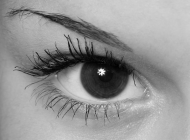
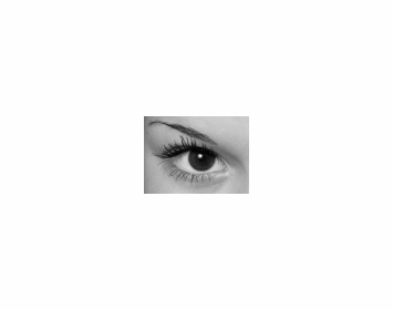
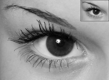
Let us now unzoom with factor $4$ a reference image, we will then rezoom it by solving problem \eqref{eq:primal-tvconstr}. The reference image eye.pgm used in this section is downloadable in PGM RAW format here (licence: CC0 public domain, source).

//* load the reference image *//
ref = readpgm('eye.pgm'); // change the path according to the location of the image on your disk.
imview(ref); //display reference
[ny,nx] = size(ref); // dimensions of domain Omega.

//* compute the dimensions of domain omega *//
z = 4;  // zoom factor = sqrt(|Omega|/|omega|)
nx0 = round(nx/z);
ny0 = round(ny/z);
z = sqrt((nx*ny)/(nx0*ny0)); // update zoom factor = sqrt(|Omega|/|omega|);

//* operator A (needed to compute u0) : unzoom operator with factor z *//
function v = A(u)
 idx = 1+z*(0:(nx0-1));
 idy = 1+z*(0:(ny0-1));
 v = zeros(ny0,nx0);
 for dx = 0:(z-1)
   for dy = 0:(z-1)
     v = v + u(dy+idy,dx+idx);
   end
 end
 v = v/z^2;
endfunction

//* compute u0 *//
u0 = A(ref);
imview(u0); // display u0

reference	$u_0$ (= reference uzoomed $\times 4$)

The $\ell^2$ projection over $A^{-1}u_0$ is given by

\begin{equation*} \forall u \in \RR^\Omega, \quad \forall (x,y) \in \Omega, \quad \pi_{A^{-1}u_0}(u)(x,y) = u(x,y) + u_0 \left( \lfloor \tfrac{x}{z} \rfloor, \lfloor \tfrac{y}{z} \rfloor\right) + A(u) \left( \lfloor \tfrac{x}{z} \rfloor, \lfloor \tfrac{y}{z} \rfloor\right)\;, \end{equation*}

where $\lfloor a \rfloor$ denotes the integer part of $a$.

This projection is easily implementable in Scilab

//* l2 projection of u over the set A^{-1}u0 = {w, Aw = u0} *//
function v = proj_constraint(u,u0)
  v = u + (u0-A(u)).*.ones(z,z);
endfunction

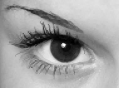
We can now run our algorithm tvconstrained to numerically solve Problem \eqref{eq:primal-tvconstr}.

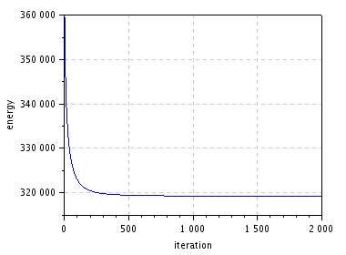
niter = 2000;
[u,E] = tvconstrained(u0,nx,ny,niter);
imview(u); // display restored image
imview(u0.*.ones(z,z)); // display details of u0
figure(); plot(1:niter,E); // plot energy evolution
xlabel("iteration"); ylabel("energy");
title("Energy decrease");

reference / $u_0$	details of $u_0$ (nearest-neighbor zoom of $u_0$)
$~$
energy decrease	restored
$~$

Spectrum extrapolation

Let us consider now the some constraints in the Fourier domain, the spectrum extrapolation method (already studied in the inverse problem framework) has been first introduced by Guichard and Malgouyres in [5]. Let us assume that the spectrum (understand here its discrete Fourier transform) of the image $u$ is known on the (small) domain $\omega$, we want to extrapolate it to the bigger domain $\Omega$.

We define $A = \tfrac{|\omega|}{|\Omega|} \cdot \mathcal{F}^{-1}_\omega \circ R_{\omega} \circ \mathcal{F}_\Omega$ in order to have

$$A u = u_0 \quad \Leftrightarrow \quad \tfrac{|\omega|}{|\Omega|} \cdot R_\omega \circ \mathcal{F}_\Omega (u) = \mathcal{F}_\omega(u_0) \;,$$

where $R_{\omega}$ denotes the restriction operator to the set $\omega$ (that is $R_{\omega} v = v_{|\omega}$, for any $v \in \RR^\Omega$), $\mathcal{F}_\Omega$ and $\mathcal{F}_\omega$ (resp. $\mathcal{F}^{-1}_\omega$) denote the direct (resp. inverse) discrete Fourier transforms of two-dimensional signals in $\RR^\Omega$ and $\RR^\omega$. The multiplicative factor $\tfrac{|\omega|}{|\Omega|}$ is used to ensure that $u$ and $u_0$ share the the same mean.

The $\ell^2$ projection over the corresponding set $A^{-1}u_0$ is simply given (in the Fourier domain) by

\begin{equation} \forall u \in \RR^\Omega, \quad \forall (\alpha,\beta) \in \Omega, \quad \tfrac{|\omega|}{|\Omega|} \cdot \mathcal{F}_\Omega \left( \pi_{A^{-1}u_0}(u) \right) (\alpha,\beta) = \left\{ \begin{array}{cl} \mathcal{F}_\omega(u_0)(\alpha,\beta) & \text{if } (\alpha,\beta) \in \omega \\ \mathcal{F}_\Omega(u)(\alpha,\beta) & \text{otherwise.} \end{array} \right. \end{equation}

Before going further, we need to discuss an important point that is usually ignored in the litterature. In general, when at least one of the dimensions of $\omega$ is even, the use of $\mathcal{F}_\omega$ and $\mathcal{F}_\omega^{-1}$ in our image processing algorithms generates nonreal values because of the dissymmetry of $\omega$ which induces in general non-Hermitian symmetry for the spectrum of manipulated images. In particular here, if $\omega$ has not two odd dimensions, we obtain in general images with nonreal values when computing $Au$ or $A^* v$ (for $u\in\RR^\Omega$ and $v \in \RR^\omega$). See this page to better understand where this phenomenon comes from and how it can be correctly handled.

For shake of simplicity, we will here simply restrict the use of the application to images $u_0$ having odd $\times$ odd dimensions.

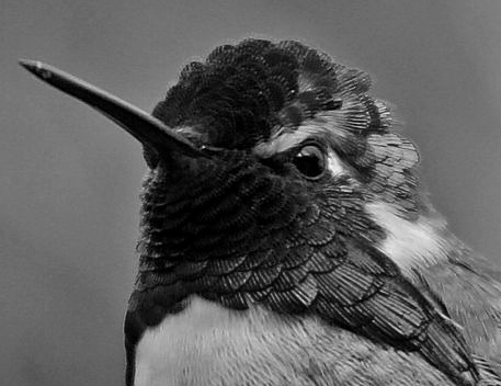
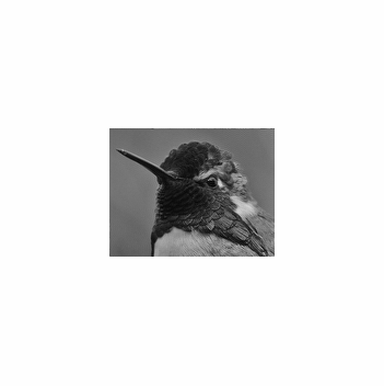
Let us now perform some numerical experiments. The reference image hummingbird.pgm used in this section is downloadable in PGM RAW format here (licence: CC0 public domain, source).

//* load the reference image *//
ref = readpgm('hummingbird.pgm'); // change the path according to the location of the image on your disk.
imview(ref); // display reference image

//* precompute Omega and omega dimensions *//
z = 3; // set the square root of the ratio |Omega|/|omega|
[ny,nx] = size(ref);
nx0 = round(nx/z);
ny0 = round(ny/z);

//* ensures omega has odd x odd dimensions *//
if(modulo(nx0,2)==0) then nx0 = nx0-1; end
if(modulo(ny0,2)==0) then ny0 = ny0-1; end
z = sqrt((nx*ny)/(nx0*ny0)); // update z = sqrt(|Omega|/|omega|)

//* define omega_x, omega_y = indexes of frequencies omega into Omega. *//
//* this allows to restrict the Fourier domain Omega to omega.         *//
omega_x = 1+modulo(nx + ifftshift((0:nx0-1)-floor(nx0/2)), nx);
omega_y = 1+modulo(ny + ifftshift((0:ny0-1)-floor(ny0/2)), ny);

//* compute and display the observed image u0 *//
dft_ref = fft(ref);
u0 = 1/z^2 * real(ifft(dft_ref(omega_y,omega_x)));
imview(u0);

reference image	observed image $u_0$ ($\sigma=2$)

Let us compute in Scilab the $\ell^2$ projection $\pi_{A^{-1}u_0}$

function v = proj_constraint(u,u0)
  dft_v = fft(u);
  dft_v(omega_y,omega_x) = z^2*fft(u0);
  v = real(ifft(dft_v));
endfunction

we can now use our tvconstrained algorithm to compute a solution of \eqref{eq:primal-tvconstr}.

niter = 500;
[u,E] = tvconstrained(u0,nx,ny,niter);
imview(u); // display restored image
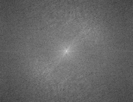
imview(fftshift(log(1+abs(fft(u))))); // display log(1+Fourier-modulus) of the restored image
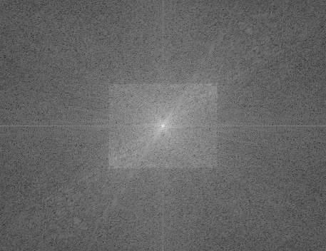
imview(fftshift(log(1+abs(fft(ref))))); // display log(1+Fourier-modulus) of the reference image
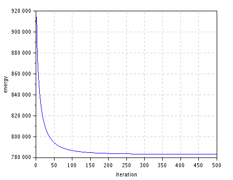
figure(); plot(1:niter,E); // plot energy evolution
xlabel("iteration"); ylabel("energy");
title("Energy decrease");

reference image	restored image

Log(1+Fourier-modulus)	Log(1+Fourier-modulus)

References

- Rudin, L. I., Osher, S., and Fatemi, E.: ``Nonlinear total variation based noise removal algorithms'', Physica D 60(1), pp. 259–268, 1992.
- Ekeland, I., and Témam, R.: ``Convex analysis and variational problems'', volume 28 of Classics in Applied Mathematics. Society for Industrial and Applied Mathematics (SIAM), Philadelphia, PA, english edition, 1999. Translated from the French.
- Chambolle, A., Pock, T.: ``A first-order primal-dual algorithm for convex problems with applications to imaging'', Journal of Mathematical Imaging and Vision, vol. 40, pp. 120–145, 2011.
- Chambolle, A., Caselles, V., Cremers, D., Novaga, M., and Pock, T.: `` An introduction to total variation for image analysis'', Theoretical foundations and numerical methods for sparse recovery, 9, 263–340, 2010.
- Guichard, F., and Malgouyres, F.: ``Total variation based interpolation'', In Proceedings of the European signal processing conference, vol. 3, pp. 1741–1744, 1998.
- Malgouyres, F., and Guichard, F.: ``Edge direction preserving image zooming: a mathematical and numerical analysis'', SIAM Journal on Numerical Analysis, vol. 39(1), pp. 1–37, 2001.
- Nikolova, M.: ``Local Strong Homogeneity of a Regularized Estimator'', SIAM Journal on Applied Mathematics, vol. 61, pp. 633–658, 2000.
- Chan, T. F., Marquina, A., and Mulet, P.: ``Higher Order Total Variation-Based Image Restoration'', SIAM Journal on Scientific Computing, vol. 22, pp. 503–516, 2000.
- Ring, W.: ``Structural Properties of Solutions to Total Variation Regularization Problems'', M2AN, Modélisation Mathématique et Analyse Numérique, vol. 34, pp. 799–810, 2000.