Inverse problem with quadratic data-fidelity and total variation regularity
Table of Contents
General formulation
Let \(u: \Omega \mapsto \RR\) denotes an (unobserved) image with discrete domain \(\Omega\) (a rectangular subset of \(\ZZ^2\)), instead of \(u\) assume that we are only able to observe a noisy version of \(Au\), where \(A: \RR^\Omega \mapsto \RR^\omega\) (\(\omega\) being another rectangular subset of \(\ZZ^2\)) is a linear operator that may model for instance the convolution with the point spread function of an acquisition sensor but also other linear observation mechanisms such as tomography, downsampling, etc.
We note \(u_0: \omega \to \RR\) the observed image, according to the observation model mentionned above, we have
$$\forall (x,y) \in \Omega, \quad u_0(x,y) = Au(x,y) + n(x,y)$$
where the \(n(x,y)\) are some realizations of independant Gaussian random variables with zero-mean and variance \(\sigma^2\). The corresponding probability density function (p.d.f) is given by
$$p(u_0 \,|\,u) = \tfrac{1}{\sigma \sqrt{2\pi}}^{|\omega|} \exp{\left( -\frac{\|Au-u_0\|_2^2}{2\sigma^2} \right)} \;.$$
As in the pure denoising case, using the improper (discrete) \(\TV\) prior \(p(u) \propto e^{-\beta \TV(u)}\) (for a given \(\beta >0\)) for natural images we get thanks to the Bayes rule the posterior density
$$p(u \, | \, u_0) \propto p(u \,|\, u_0) \, p(u) = \exp{\left( -\frac{\|Au-u_0\|_2^2}{2\sigma^2} - \beta \TV(u) \right)}\;,$$
the notation \(\propto\) indicates an equality up to a multiplicative constant (that may depend on \(u_0\) but not \(u\)).
The Maximum A Posteriori approach (MAP) consists in computing the image that maximizes the posterior density \(p(u \,|\,u_0)\) or equivalently that mininimizes the convex energy \(-\log{p(u \,|\, u_0)}\), leading to the inverse problem
\begin{equation} \label{eq:primal-inverse} % \widehat{u}_\text{MAP} = \arg \, \min_{u \in \RR^\Omega} \tfrac{1}{2} \| Au-u_0 \|_2^2 + \lambda \TV(u) % \end{equation}where \(\lambda = \beta \sigma^2\) denotes the regularity parameter (that must be set by the user).
Primal-dual reformulation
Dual of the regularity term
Recall the dual formulation of the discrete total variation (see here the page dedicated to the discrete total variation)
\begin{equation} \label{eq:dual-tv} % \TV(u) = \max_{p \in \RRRR{\Omega}} \langle \nabla u , p \rangle \quad \text{subject to} \quad \|p\|_{\infty,2} \leq 1 \;, % \end{equation}where \(\|p\|_{\infty,2} = \max_{(x,y) \in \RR^\Omega} \|p(x,y)\|_2\).
Dual of the data fidelity term
Let \(f: v \in \RR^\omega \to \tfrac{1}{2} \|v-u_0\|_2^2\), so that the data fidelity term in \eqref{eq:primal-inverse} is \(f(Au) = \tfrac{1}{2} \| Au -u_0 \|_2^2\). Since \(f\) is a convex and lower semi-continuous function (in other words, an element of \(\Gamma(\RR^\omega)\)), we have
$$\forall u \in \RR^\Omega, \quad f(Au) = f^{\star\star}(Au) = \sup_{q \in \RR^\omega} \langle Au , q \rangle - f^\star(q) \;.$$
Now let \(q \in \RR^\omega\), we have
\begin{equation*} % \begin{array}{ll} f^\star(q) &=& \sup\limits_{\substack{v \in \RR^\omega}} \langle q,v \rangle - f(v) \\ &=& \sup\limits_{\substack{v \in \RR^\omega}} \langle q,v \rangle - \tfrac{1}{2} \|v-u_0\|_2^2 \\ &=& \tfrac{1}{2}\|q\|_2^2 + \langle q , u_0 \rangle + \underset{=0}{\underbrace{\sup\limits_{\substack{v \in \RR^\omega}} \tfrac{1}{2} \|v-u_0-q\|_2^2}} \\ &=& \tfrac{1}{2}\|q+u_0\|_2^2 - \tfrac{1}{2} \| u_0 \|_2^2 \;. \\ \end{array} % \end{equation*}Finally we get
\begin{equation} \label{eq:dual-fidelity} % \begin{array}{ll} f(Au) &= f^{\star\star}(Au) = \sup\limits_{\substack{q \in \RR^\omega}} \langle Au, q \rangle - \tfrac{1}{2} \|q+u_0\|_2^2 + \tfrac{1}{2} \|u_0\|_2^2 \\ &= \tfrac{1}{2} \|u_0\|_2^2 + \max\limits_{\substack{q \in \RR^\omega}} \langle Au, q \rangle - \tfrac{1}{2} \|q+u_0\|_2^2 \;, \end{array} % \end{equation}indeed the supremum is realized at point \(q=Au-u_0\), thus the supremum can be replaced by a maximum.
Primal-dual reformulation
Replacing in \eqref{eq:primal-inverse} the \(\TV\) term by \eqref{eq:dual-tv}, the data-fidelity term by \eqref{eq:dual-fidelity} and removing the constant term \(\tfrac{1}{2}\|u_0\|_2^2\) (which does not change the minimizer of \eqref{eq:primal-inverse} since this term does not depend on \(u\)), we get
\begin{equation} \label{eq:primal-dual-inverse} % \hat{u}_\text{MAP} = \arg \, \min_{u \in \RR^\Omega} \, \max\limits_{\substack{p \in \RRRR{\Omega} \\ q \in \RR^\omega}} \langle \left( \lambda \nabla u , Au \right) , (p,q) \rangle - \delta(p) - \tfrac{1}{2} \|q+u_0\|_2^2 \;, % \end{equation}where \(\delta\) denotes the indicator function of the closed unit ball of the norm \(\|\cdot\|_{\infty,2}\), that is
\begin{equation} \forall p \in \RRRR{\Omega}, \quad \delta(p) = \left\{ \begin{array}{cl} 0 & \text{if } \|p\|_{\infty,2} \leq 1 \\ +\infty & \text{otherwise.} \end{array} \right. \end{equation}We will use the Chambolle and Pock algorithm [3] to numerically solve the primal-dual problem \eqref{eq:primal-dual-inverse}.
Computational procedure
The Chambolle and Pock algorithm
A solution of problem \eqref{eq:primal-dual-inverse} can be numerically computed using the algorithm of Chambolle-Pock [3], which is designed to solve the generic saddle-point problem
\begin{equation} \label{eq:cp.primal-dual} \arg\,\min_{x \in X}\max_{y \in Y} ~ G(x) + \langle Kx , y \rangle - F^\star(y) \;. \end{equation}The algorithm is briefly presented on this page.
Taking \(X=\RR^\Omega\), \(Y=\left(\RRRR{\Omega} \right) \times \RR^\omega\), \(x=u\), \(y=(p,q)\), \(F^\star(p,q) = \delta(p) + \tfrac{1}{2}\|q+u_0\|_2^2\), \(G(u) = 0\) and \(Ku = \left(\lambda \nabla u , Au \right)\) into problem \eqref{eq:cp.primal-dual} allows to recover problem \eqref{eq:primal-dual-inverse}.
We note \(\divergence = -\nabla^*\) the opposite of the adjoint of the operator \(\nabla\) (in analogy with the continuous setting) and \(A^*\) the adjoint of \(A\), we have then \(K^* = -\lambda \divergence + A^*\). The update of the dual variable (here the tuple (p, q)) in the Chambolle-Pock algorithm (see Algorithm 1 in on this page) can been split into two independant updates thanks to the additive separability with respect to \(p\) and \(q\) of \((p,q) \to \langle K u , (p,q) \rangle - F^\star(p,q)\), hence applying the Chambolle and Pock algorithm to problem \eqref{eq:cp.primal-dual} boils down to Algorithm 1.
Chambolle-Pock resolvant algorithm for problem \eqref{eq:primal-dual-inverse}.
Initialization: Choose \(\tau, \sigma > 0\), \(\theta \in [0,1]\), \(u^0 \in \RR^\Omega\), \(p^0 \in \RRRR{\Omega}\), \(q^0 \in \RR^\omega\) and set \(\bar{u}^0 = u^0\).
Iterations (\(k \geq 0\)): Update \(u^k\), \(p^k\), \(q^k\) and \(\bar{u}^k\) as follows
\begin{eqnarray} p^{k+1} &=& \arg\,\min\limits_{\substack{p \in \RRRR{\Omega} }} ~ \tfrac{1}{2\sigma} \left\|p-(p^k+\sigma \lambda \nabla \bar{u}^k)\right\|_2^2 + \delta(p) \label{cp.dual-p} \\ q^{k+1} &=& \arg\,\min\limits_{\substack{q \in \RR^\omega }} ~ \tfrac{1}{2\sigma} \left\|q-(q^k+\sigma A \bar{u}^k)\right\|_2^2 + \tfrac{1}{2} \|q+u_0\|_2^2 \label{cp.dual-q} \\ u^{k+1} &=& \arg\,\min\limits_{\substack{u \in \RR^\Omega}} ~ \tfrac{1}{2\tau} \left\|u-\left(u^k +\tau \lambda \divergence p^{k+1} - \tau A^* q^{k+1}\right)\right\|_2^2 \label{cp.primal} \\ \bar{u}^{k+1} &=& u^{k+1} + \theta \left(u^{k+1}-u^{k}\right) \nonumber \end{eqnarray}\(~\)
The dual and primal updates (Equations \eqref{cp.dual-p}, \eqref{cp.dual-q} and \eqref{cp.primal}) can be computed in closed-form.
The first dual update \eqref{cp.dual-p} boils down to the pointwise operations $$ % \forall (x,y) \in \Omega, \quad p^{k+1}(x,y) = \frac{p^k(x,y) + \sigma \lambda \nabla \bar{u}^k(x,y) }{\max { \left( 1 , \left|\, p^k(x,y) + \sigma \lambda \nabla \bar{u}^k(x,y) \,\right|_2 \right) }} \;, % $$ the second dual update \eqref{cp.dual-q} boils down th to pointwise operations $$ % \forall (x,y) \in \omega, \quad q^{k+1}(x,y) = \frac{q^k(x,y)+\sigma \left( A \bar{u}^k(x,y) - u_0(x,y) \right)}{1+\sigma} \;, % $$ and the primal update \eqref{cp.primal} boils down to the pointwise operations $$ \forall (x,y) \in \Omega, \quad u^{k+1}(x,y) = u^k +\tau \lambda \divergence p^{k+1} - \tau A^* q^{k+1} \;. $$
Notice that the convergence of Algorithm 1 toward the (here unique) solution of problem \eqref{eq:primal-dual-inverse} is ensured when \(\theta = 1\) and \(\tau \sigma {|||K|||}^2 < 1\). Here we have \({|||K|||}^2 \leq \lambda^2 {|||\nabla|||}^2 + {|||A|||}^2\), this upper bound depends on the choice of the operator \(A\) and the discretization scheme used for \(\nabla\).
Discretization schemes
Let \(n_x\) and \(n_y\) denote the width and height of the initial (noisy) image \(u_0\), we note \(\Omega = \left\{ 1, \dots , n_x \right\} \times \left\{ 1, \dots , n_y \right\}\) the discrete domain of \(u_0\). We propose here to use the following finite difference scheme for the gradient operator
$$ \forall u \in \RR^\Omega, \quad \forall (i,j) \in \Omega, \quad \nabla u (i,j) = \left( \nabla_x u (i,j), \nabla_y u (i,j) \right)\;, $$
where
\begin{equation*} % \nabla_x u (i,j) = \left\{ \begin{array}{cl} u(i+1,j) - u(i,j) & \text{if } i < n_x \\ 0 & \text{if } i=n_x \end{array} \right. % \quad % \nabla_y u (i,j) = \left\{ \begin{array}{cl} u(i,j+1) - u(i,j) & \text{if } j < n_y \\ 0 & \text{if } j = n_y \end{array} \right. % \end{equation*}This operator is easily implementable in Scilab langage,
function [Dx,Dy] = grad(u)
  [ny,nx] = size(u);
  Dx = u(:,[2:nx,nx]) - u;
  Dy = u([2:ny,ny],:) - u;
endfunction
and we can prove that the corresponding divergence operator (the opposite of the adjoint of \(\nabla\)) is given by
$$ \forall p = (p_x,p_y) \in \RRRR{\Omega}, \quad \forall (i,j) \in \Omega, \quad \divergence{(p)}(i,j) = \text{div}_x (p_x)(i,j) + \text{div}_y (p_y)(i,j) \;, $$
where
\begin{equation*} % \text{div}_x (p_x)(i,j) = \left\{ \begin{array}{cl} p_x(i,j)-p_x(i-1,j) & \text{if } 1 < i < n_x \\ p_x(i,j) & \text{if } i = 1 \\ -p_x(i-1,j) & \text{if } i = n_x \\ \end{array} \right. % \quad % \text{div}_y (p_y)(i,j) = \left\{ \begin{array}{cl} p_y(i,j)-p_y(i,j-1) & \text{if } 1 < j < n_y \\ p_y(i,j) & \text{if } j = 1 \\ -p_y(i,j-1) & \text{if } j = n_y \\ \end{array} \right. \end{equation*}This operator is also easily implementable in Scilab langage.
function d = div(px,py) // compute d = div(p) where p = (px,py) and size(px) == size(py)
  [ny,nx] = size(px);
  div_x      =  px - px(:,[1,1:(nx-1)]);
  div_x(:,1) =  px(:,1);
  div_x(:,nx) = -px(:,nx-1);
  div_y      =  py - py([1,1:(ny-1)],:);
  div_y(1,:) =  py(1,:);
  div_y(ny,:) = -py(ny-1,:);
  d = div_x + div_y;
endfunction
Scilab implementation of the Chambolle Pock algorithm
With the choice of discretization scheme described in the previous section, we can show that the induced \(\ell^2\) norm of the operator \(\nabla\) is less than \(\sqrt{8}\) (that is \({|||\nabla|||} \leq \sqrt{8}\)). Let us note \(L_A\) an upper bound of \({|||A|||}\) (will be precised for each application proposed), we have \({|||K|||} \leq L := \sqrt{8\lambda^2 + L_A^2}\), therefore taking \(\tau = \sigma = \tfrac{0.99}{L}\) into Algorithm 1 ensures that \(\tau \sigma \, {|||K|||}^2 < 1\) (which, in addition to the setting \(\theta=1\) is sufficient to ensure the convergence of the algorithm toward the solution of problem \eqref{eq:primal-inverse}).
We propose below a Scilab implementation of Algorithm 1 that can be used to solve the inverse problem \eqref{eq:primal-inverse} once the operator \(A\), its adjoint \(A^*\) and an upper bound \(L_A\) of \(|||A|||\) are set into Scilab memory.
More precisely, the user must fill according to the intended application, the following code and load it into Scilab memory
//* define operator A *//
function v = A(u)
  //* enter your code here *//
  ...
endfunction

//* define adjoint of A *//
function u = adj_A(v)
  //* enter your code here *//
  ...
endfunction

//* define an upperbound for the induced l2 norm of A *//
L_A = ... //* enter the value here *//
optionally, the user may define an initial value for the primal variable \(u\)
(initializing the algorithm with a more or less good guess of the solution may
drastically accelerate the convergence). For that simply load into Scilab
memory the initialization of your choice with the name init. If this init
is not defined the primal variable \(u\) will be initialized to the null image
(image full of zeros).
init = ... //* enter the value here *//
Once the setting is done, you can use the following implementation of Algorithm 1 to solve the inverse problem with the Chambolle and Pock algorithm.
 //          Solver for inverse problems with quadratic data-fidelity
 //                     and total variation regularity
 //
 // u0 = input image
 // lambda = regularity parameter (TV weight)
 // niter = number of iterations for the Chambolle-Pock algorithm
 // u = restored image
 // E = energy (E(i) = energy computed at iteration i)
 //
 // Warning: the bound L_A and the operators A, adj_A must have been
//           defined into Scilab memory.
 function [u,E] = inverse_solver_tvreg(u0,lambda,niter)

   E = zeros(1,niter);

   // retrieve dimensions of domains omega & Omega (recall
   // that operator A is from R^Omega to R^omega).
   [ny0,nx0] = size(u0);      // domain omega
   [ny,nx] = size(adj_A(u0)); // domain Omega

   // initialize primal and dual variables
   if(exists("init")) then
     if((size(u,1) == ny)&(size(u,2) == nx)) then u = init;
     else u = zeros(ny,nx); end
   else u = zeros(ny,nx); end
   ubar = u;
   px = zeros(u);
   py = zeros(u);
   q = zeros(ny0,nx0);

   // set Chambolle & Pock algorithm time-step parameters
   L = sqrt(8*lambda^2+L_A^2);
   tau = 0.99/L;
   sigma = 0.99/L;
   theta = 1;

   //**************************** main loop ****************************//
   for i = 1:niter
     //* compute (Dx,Dy) = grad(ubar) *//
     [Dx,Dy] = grad(ubar);
     //* update p = (px,py) *//
     px  = px + sigma*lambda*Dx;
     py  = py + sigma*lambda*Dy;
     nrm = px.*px + py.*py;
     id = nrm > 1; nrm = sqrt(nrm(id));
     px(id) = px(id) ./ nrm;
     py(id) = py(id) ./ nrm;
     //* update q *//
     q = (q + sigma*(A(ubar)-u0))/(1+sigma);
     //* compute d = div(p) *//
     d = div(px,py);
     //* update u and ubar *//
     ubar = -theta * u;
     u    = u + tau*(lambda*d-adj_A(q));
     ubar = ubar + (1+theta)*u;
     //* compute energy of u *//
     [Dx,Dy] = grad(u);
     tv = sum(sqrt(Dx.^2 + Dy.^2));
     E(i) = 0.5*sum((A(u)-u0).^2) + lambda*tv;
     printf("iteration %d : E = %.10g\n",i,E(i));
   end
   //************************* end of main loop *************************//
 endfunction
Applications
Basic tools for image manipulation in Scilab
We first propose some very basic tools dedicated to image manipulation in Scilab (opening, visualization).
Image viewer
function imview(u)
  [height,width] = size(u);
  fg = figure();
  set(fg,"axes_size",[width,height],"infobar_visible","on","menubar_visible","on","toolbar_visible","off","auto_resize","off","color_map",graycolormap(256));
  set(fg.children,"margins",zeros(1,4));
  Matplot(255/(%eps + max(u)-min(u)) * (u-min(u)),"010",[1,1,width,height]);
endfunction
Image opening (format PMG)
// open a PGM RAW image (8 bits)
// usage: u = readpgm('lena.pgm');
function image=readpgm(filename)
  //* local function *//
  function l=getline(u)
    h=[]
    while %t
      c=mget(1,'uc',u)
      if c==10 then break, end
      h=[h c]
    end
    l=ascii(h)
  endfunction
  //* main *//
  [u,err]=mopen(filename,'rb')
  if err<>0 then error('Impossible to open file '+filename), end
  if getline(u)~='P5' error('Unrecognized format'), end
  z=getline(u), while part(z,1)=='#', z=getline(u), end
  execstr('n=['+z+']')
  getline(u)
  image=matrix(mget(n(1)*n(2),'uc',u),n)'
  mclose(u)
endfunction
Image deconvolution (application to deblurring)
In the case of image deconvolution, the linear operator \(A\) in \eqref{eq:primal-inverse} is the convolution with a point spread function (modeling for instance some blurring phenomena such as diffraction, defocus or motion, etc.). Notice that a convolution can only model uniform phenomena while in practice optical devices generally suffer from more complicated distortions such as chromatic aberrations, stigmatism and coma, vignetting, etc. The correction of such non-uniform distortions is therefore out of the scope of the restoration application detailed here.
Let us consider a discrete convolution kernel \(k_A \in \RR^{\omega_A}\) with domain \(\omega_A \subset \ZZ^2\) that we can assume to be symmetric (\((a,b) \in \omega_A \Leftrightarrow (-a,-b) \in \omega_A\)) without loss of generality. We define \(A : \RR^\Omega \mapsto \RR^\omega\) by
\begin{equation} \label{eq:discrete_convol} \forall (x,y) \in \omega, \quad Au(x,y) = \sum_{(a,b) \in \omega_A} k_A(a,b) \, u(x-a,y-b)\;, \end{equation}and \(\omega\) denotes the subset of \(\Omega\) made of all the pixels \((x,y) \in \Omega\) such as \((x,y)-\omega_A \subset \Omega\). Remark that it is also possible to define the convolution with kernel \(k_A\) as an operator \(A : \RR^\Omega \mapsto \RR^\Omega\) at the cost of an extension of \(u\) outside of \(\Omega\), usually a periodic or nearest-neighbour recopy, or a zero-extension of the image \(u\) is considered, which is of course nonrealistic in most situations.
In order to use the Scilab implementation inverse_solver_tvreg,
we need to compute the adjoint \(A^*\) and an upper bound of \(|||A|||\).
The adjoint of the operator \(A\) defined in \eqref{eq:discrete_convol} is the operator \(A^* : \RR^\omega \mapsto \RR^\Omega\) defined by $$ % \forall v \in \RR^\omega, \quad \forall (x,y) \in \Omega, \quad A^*v (x,y) = \sum_{(a,b) \in \omega_A} k_A(a,b) \, v(x+a,y+b)\;, % $$ with the convention that \(v(x+a,y+b)=0\) when \((x+a,y+b) \not\in \omega\).
The induced \(\ell^2\) norm of \(A\) is bounded from above by \(\|k_A\|_1\).
The first assertion is straightforward, simply check that \(\forall (u,v) \in \RR^\Omega \times \RR^\omega\) we have \(\langle Au,v \rangle = \langle u,A^* v\rangle\). Let us detail the second assertion. For any image \(u \in \RR^\Omega\), we have
\begin{equation*} \begin{array}{ll} \|Au\|_2 &= \displaystyle{\max_{v \in \RR^\omega,~ \|v\|_2 \leq 1}} \langle v, Au \rangle \\ &= \displaystyle{\max_{v \in \RR^\omega,~ \|v\|_2 \leq 1}} \sum_{(x,y) \in \omega} \sum_{(a,b) \in \omega_A} v(x) \, k_A(a,b) \, u(x-a,y-b) \\ &= \displaystyle{\sum_{(a,b) \in \omega_A}} \displaystyle{\max_{v \in \RR^\omega,~ \|v\|_2 \leq 1}} \sum_{(x,y) \in \omega} v(x,y) \, k_A(a,b) \, u(x-a,y-b) \\ &= \displaystyle{\sum_{(a,b) \in \omega_A}} \displaystyle{\max_{v \in \RR^\omega,~ \|v\|_2 \leq 1}} \langle v , k_A(a,b) \, u(\cdot-a,\cdot-b) \rangle \\ &= \displaystyle{\sum_{(a,b) \in \omega_A}} \left|k_A(a,b)\right| \cdot \|u(\cdot-a,\cdot-b)\|_2 \;, \end{array} \end{equation*}where \(u(\cdot-a,\cdot-b) = \left( (x,y) \in \omega \to u(x-a,y-b) \right)\). As for any \((a,b) \in \omega_A\) we have \(\|u(\cdot-a)\|_2 \leq \|u\|_2\) (the left-hand norm is the \(\ell^2\) norm over \(\RR^\omega\) and the right-hand is the \(\ell^2\) norm over \(\RR^\Omega\)), we get the upper bound \(\|Au\|_2 \leq \|k_A\|_1 \cdot \|u\|_2\) and thus \(|||A||| \leq \|k_A\|_1\).
We can now implement those operators in Scilab, actually thanks to the built-in
conv2 function, the code is straightforward. The (motion) blur kernel used for
this experiment can be downloaded here in sod format (Scilab variable storing
format).
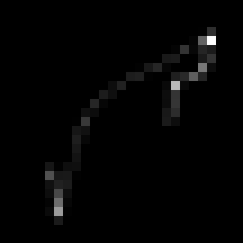
load('motion_kernel.sod') ; // load the variable "ker" (a motion blur kernel) into Scilab memory...
// ...or define your own kernel, for instance: "ker = ones(5,5)/25;"
imview(ker.*.ones(10,10)); // visualize kernel (zoom x10)

//* set operator A = convolution with kernel "ker" *//
function v = A(u)
  v = conv2(u,ker,"valid");
endfunction

//* define the adjoint of A *//
ker_sym = ker($:-1:1,$:-1:1);
function u = adj_A(v)
  u = conv2(v,ker_sym,"full");
endfunction

//* set an upper bound for |||A||| *//
L_A = sum(abs(ker));
| motion kernel (size 27 \(\times\) 27) |
 |
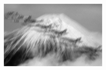
Let us now compute a blurry and noisy observation of a reference image.
The reference image fuji.pgm used in this section is downloadable in
PGM RAW format here (licence: CC0 public domain, source).
ref = readpgm('fuji.pgm'); // change the path according to the location of the image on your disk.
imview(ref);
sigma = 2;
u0 = A(ref);
u0 = u0 + grand(u0,'nor',0,sigma);
imview(u0);
| reference image (domain \(\Omega\)) | \(u_0\) blurry and noisy observation (domain \(\omega\)) |
 \(~\) \(~\) |
 |
Before running the algorithm, we suggest to use an initialization (this is optional but drastically reduce the number of iteration necessary to reach convergence). The input (\(u_0\)) of the algorithm has domain \(\omega\), the output (\(u\)) has domain \(\Omega\). We propose to extend \(u_0\) to the domain \(\Omega\) with a Neumann boundary condition (that is pixel recopy at the frontier of \(\omega\)) and use this extended image as initializer.
// compute init = u0 extended to domain Omega with pixel recopy
// boundary condition (drastically improve convergence speed)
[ny0,nx0] = size(u0);
dx = floor((size(ker,2)-1)/2);
dy = floor((size(ker,1)-1)/2);
init = u0([ones(1,dy),1:ny0,ny0*ones(1,dy)],[ones(1,dx),1:nx0,nx0*ones(1,dx)]);
We are now ready to use inverse_solver_tvreg to solve problem
\eqref{eq:primal-inverse} with the Chambolle and Pock algorithm.
lambda = 0.2;
niter = 200;
[u,E] = inverse_solver_tvreg(u0,lambda,niter);
imview(u); // display output (restored)
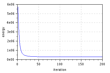
figure(); plot(1:niter,E); // plot energy evolution
xlabel("iteration"); ylabel("energy");
title("Energy decrease");
| reference | blurry and noisy (\(\sigma = 2\)) |
 \(~\) \(~\) |
 |
| restored (\(200\) iterations, \(\lambda=0.2\)) | energy decrease |
 \(~\) \(~\) |
 |
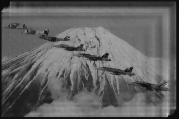
To illustrate how we benefit from a good initialization, let us run the algorithm taking the null image as initializer for the primal variable \(u\),
init = zeros(ref);
lambda = 0.2;
v200  = inverse_solver_tvreg(u0,lambda,200);  // niter =  200
v2000 = inverse_solver_tvreg(u0,lambda,2000); // niter = 2000
v5000 = inverse_solver_tvreg(u0,lambda,5000); // niter = 5000
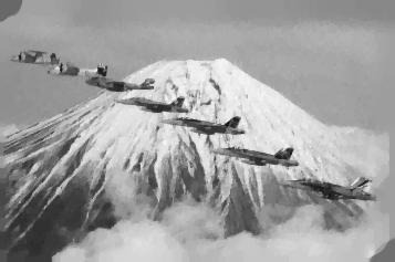
| null initialization, 200 iterations | null initialization, 2000 iterations |
 \(~\) \(~\) |
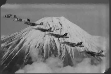 |
| null initialization, 5000 iterations | null initialization, 10000 iterations |
 \(~\) \(~\) |
 |
Image zooming
The inverse problem \eqref{eq:primal-inverse} can also be used to perform image zooming (see [6,3]). For such application, the operator \(A\) is oftenly assumed to be a blurring kernel followed by a subsampling procedure.
We consider two discrete domains, a (small) domain \(\omega = \left[ 0, M \right) \times \left[ 0, N \right) \cap \ZZ^2\), and a (bigger) domain \(\Omega = \left[ 0, z M \right) \times \left[ 0, z N \right) \cap \ZZ^2\), where \(z\) denotes a given positive integer (zoom factor). We set \(\omega_A = \left[0,z\right) \times \left[0, z\right) \cap \ZZ^2\) and define \(A: \RR^\Omega \mapsto \RR^\omega\) by
\begin{equation} \label{eq:captor_integration} \forall u \in \RR^\Omega, \quad \forall (x,y) \in \omega, \quad Au(x,y) = \frac{1}{z^2} \sum_{(a,b) \in \omega_A} u(zx+a, zy+b)\;. \end{equation}Remark that \(Au\) is nothing more than a zero order unzoom with factor $z of the image \(u\), it consists in partitioning \(\Omega\) into square cells \(\omega_A\) and to average \(u\) over each one of the cells. The operator \(A\) can also be seen as a discrete approximation of a captor integration procedure, wich models the photon count averaging process that is done over the (in reality continuous) square domain \(\left[ 0, z \right) \times \left[ 0, z \right)\) of each captor covering the focal plane of the image acquisition system (for instance for CCD or CMOS cameras).
The unzoom operator \(A\) defined in \eqref{eq:captor_integration} has induced \(\ell^2\) norm bounded by \(|||A||| \leq \tfrac{1}{z}\) and its adjoint is the operator \(A^* : \RR^\omega \mapsto \RR^\Omega\) defined by $$ % \forall v \in \RR^\Omega, \quad \forall (x,y) \in \Omega, \quad A^*v (x,y) = \frac{1}{z^2} \, v \left( \lfloor \tfrac{x}{z} \rfloor , \lfloor \tfrac{y}{z} \rfloor \right) \;, % $$ where \(\lfloor a \rfloor\) denotes the integer part of \(a\).
Let us now define those operators into Scilab memory.
//* set A operator = unzoom with factor z *//
z = 4; // set unzoom factor
function v = A(u)
  [ny,nx] = size(u);
  nx0 = nx/z; // warning: must be an integer
  ny0 = ny/z; // warning: must be an integer
  idx = 1+z*(0:(nx0-1));
  idy = 1+z*(0:(ny0-1));
  v = zeros(ny0,nx0);
  for dx = 0:(z-1)
    for dy = 0:(z-1)
      v = v + u(dy+idy,dx+idx);
    end
  end
  v = v/z^2;
endfunction

//* define the adjoint of A *//
k = ones(z,z)/z^2;
function u = adj_A(v)
  u = v .*. k;
endfunction

//* set an upper bound for |||A||| *//
L_A = 1/z;
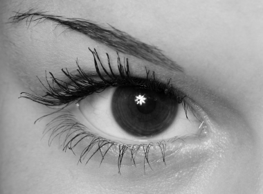
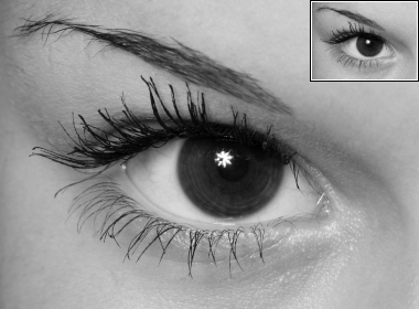
Let us now unzoom with factor \(4\) a reference image, we will then
rezoom it by solving problem \eqref{eq:primal-inverse}. The
reference image eye.pgm used in this section is downloadable
in PGM RAW format here (licence: CC0 public domain, source).
ref = readpgm('eye.pgm'); // change the path according to the location of the image on your disk.
imview(ref);
sigma = 2;
u0 = A(ref);
u0 = u0 + grand(u0,'nor',0,sigma);
imview(u0);
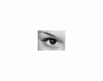
| reference | unzoomed (\(\times 4\)) and noisy (\(\sigma = 2\)) |
 |
 |
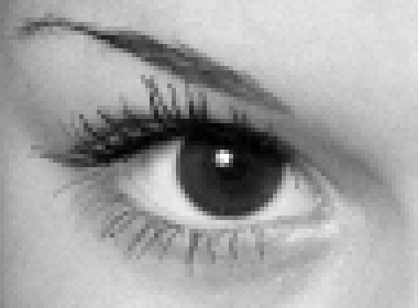
Now let us use inverse_solver_tvreg to solve problem
\eqref{eq:primal-inverse}, we will use as initializer a
nearest neighbor zoom of \(u_0\).
niter = 2000;
lambda = 0.2;
init = u0.*.ones(z,z); // set init = nearest neighbor zoom of factor z of u0.
[u,E] = inverse_solver_tvreg(u0,lambda,niter);
imview(u); // display output (restored)
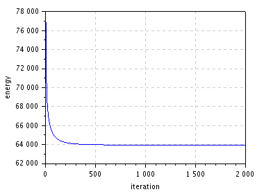
figure(); plot(1:niter,E); // plot energy evolution
xlabel("iteration"); ylabel("energy");
title("Energy decrease");
| reference / \(u_0\) | details of \(u_0\) (nearest-neighbor zoom of \(u_0\)) |
 \(~\) \(~\) |
 |
| energy decrease | restored (\(\lambda = 0.2\)) |
 \(~\) \(~\) |
 |
Thanks to Scilab built-in functions, we can easily rezoom \(u_0\) using the bicubic spline interpolation.
//* zoom u0 using bicubic spline interpolation *//
[ny0,nx0] = size(u0);
x = 0:(nx0-1);
y = 0:(ny0-1);
C = splin2d(y,x,u0,"natural");
xx = linspace(0,nx0-1,z*nx0);
yy = linspace(0,ny0-1,z*ny0);
[XX,YY] = ndgrid(xx,yy);
z_bicubic = (interp2d(YY,XX, y, x, C, "natural"))';
imview(z_bicubic);
| bicubic spline zoom (\(\times 4\)) of \(u_0\) | \(\TV\) restored (\(\lambda = 0.2\)) |
 \(~\) \(~\) |
 |
The total variation based zooming yields much sharper image but clearly suffers to much from staircasing effect (that is the creation of flat region with artificial boundaries in the restored image) and from a strong block effect. We will see that the use of the Huber total variation allows to get rid of this undesirable artifact, but will not reduce the appearance of blocks. Those blocks are favored by the fidelity term in \eqref{eq:primal-inverse} (due to the particular structure of the operator \(A\) that we try to inverse, indeed \(Au\) is obtained by averaging \(u\) over non-overlapping square cells of size \(z \times z\)) and are not penalized by the \(\TV\) regularizer which is not very sensitive to sharp horizontal and vertical edges.
Spectrum extrapolation
The spectrum extrapolation method has been first introduced by Guichard and Malgouyres in [5]. Let us assume that the spectrum (understand here its discrete Fourier transform) of the image \(u\) is known on the (small) domain \(\omega\), we want to extrapolate it to the bigger domain \(\Omega\).
We define \(A = \tfrac{|\omega|}{|\Omega|} \cdot \mathcal{F}^{-1}_\omega \circ R_{\omega} \circ \mathcal{F}_\Omega\) in order to have
$$A u = u_0 \quad \Leftrightarrow \quad \tfrac{|\omega|}{|\Omega|} \cdot R_\omega \circ \mathcal{F}_\Omega (u) = \mathcal{F}_\omega(u_0) \;,$$
where \(R_{\omega}\) denotes the restriction operator to the set \(\omega\) (that is \(R_{\omega} v = v_{|\omega}\), for any \(v \in \RR^\Omega\)), \(\mathcal{F}_\Omega\) and \(\mathcal{F}_\omega\) (resp. \(\mathcal{F}^{-1}_\omega\)) denote the direct (resp. inverse) discrete Fourier transforms of two-dimensional signals in \(\RR^\Omega\) and \(\RR^\omega\). The multiplicative factor \(\tfrac{|\omega|}{|\Omega|}\) is used to ensure that \(u\) and \(u_0\) share the the same mean.
The adjoint of \(A\) is the operator \(A^* : \RR^\omega \mapsto \RR^\Omega\) defined in the Fourier domain by
\begin{equation*} \forall v \in \RR^\omega, \quad \forall (\alpha,\beta) \in \omega, \quad \mathcal{F}_\Omega (A^* v)(\alpha,\beta) = \left\{ \begin{array}{cl} \mathcal{F}_\omega(v)(\alpha,\beta) & \text{if } (\alpha,\beta) \in \omega \\ 0 & \text{otherwise.} \end{array} \right. \end{equation*}Besides, we have \({|||A|||} \leq 1\).
Notice that in [5], Guichard and Malgouyres are interested in computing the image \(u\) with smallest total variation among those satisfying the constraint \(Au = u_0\), that is
\begin{equation} \label{eq:tvextrap} \widehat{u} = \arg \, \min_{u \in \RR^\Omega} \TV(u) \quad \text{subject to} \quad Au = u_0 \;, \end{equation}The resolution of such problem is adressed in this page dedicated to the resolution of constrained minimization of the total variation). Instead of \eqref{eq:tvextrap} we consider here the relaxed version given by problem \eqref{eq:primal-inverse}, which amounts to compute the image that satisfy a good compromise between two requirements: "having a small total variation" and "verifying Au ≈ u0".
Before going further, we need to discuss an important point that is usually ignored in the litterature. In general, when at least one of the dimensions of \(\omega\) is even, the use of \(\mathcal{F}_\omega\) and \(\mathcal{F}_\omega^{-1}\) in our image processing algorithms generates nonreal values because of the dissymmetry of \(\omega\) which induces in general non-Hermitian symmetry for the spectrum of manipulated images. In particular here, if \(\omega\) has not two odd dimensions, we obtain in general images with nonreal values when computing \(Au\) or \(A^* v\) (for \(u\in\RR^\Omega\) and \(v \in \RR^\omega\)). See this page to better understand where this phenomenon comes from and how it can be correctly handled.
For shake of simplicity, we will here simply restrict the use of the application to images \(u_0\) having odd \(\times\) odd dimensions.
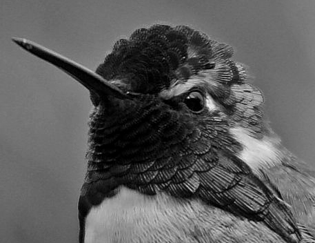
Let us now configure our inverse_solver_tvreg algorithm to
perform spectrum extrapolation. The reference image
hummingbird.pgm used in this section is downloadable
in PGM RAW format here (licence: CC0 public domain, source).
//* load the reference image *//
ref = readpgm('hummingbird.pgm'); // change the path according to the location of the image on your disk.

//* precompute Omega and omega dimensions *//
z = 3; // set the square root of the ratio |Omega|/|omega|
[ny,nx] = size(ref);
nx0 = round(nx/z);
ny0 = round(ny/z);

//* ensures omega has odd x odd dimensions *//
if(modulo(nx0,2)==0) then nx0 = nx0-1; end
if(modulo(ny0,2)==0) then ny0 = ny0-1; end
z = sqrt((nx*ny)/(nx0*ny0)); // update z = sqrt(|Omega|/|omega|)


//* define omega_x, omega_y = indexes of frequencies omega into Omega. *//
//* this allows to restrict the Fourier domain Omega to omega.         *//
omega_x = 1+modulo(nx + ifftshift((0:nx0-1)-floor(nx0/2)), nx);
omega_y = 1+modulo(ny + ifftshift((0:ny0-1)-floor(ny0/2)), ny);

//* define operator A *//
function v = A(u)
  dft_u = fft(u);
  dft_v = dft_u(omega_y,omega_x);
  v = 1/z^2 * real(ifft(dft_v));
endfunction

//* define the adjoint of A *//
function u = adj_A(v)
  dft_u = zeros(ny,nx);
  dft_u(omega_y,omega_x) = fft(v);
  u = real(ifft(dft_u));
endfunction

//* set an upper bound for |||A||| *//
L_A = 1;
We compute now a noisy observation \(u_0\) of the reference image.
sigma = 2; // set the level of noise
u0 = A(ref) + grand(ny0,nx0,'nor',0,sigma);
imview(ref); // display reference image
imview(u0); // display observed image
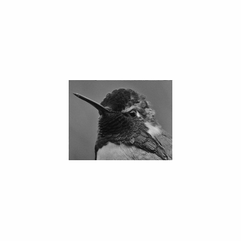
| reference image | observed image \(u_0\) (\(\sigma=2\)) |
 |
 |
Let us run our inverse_solver_tvreg algorithm.
lambda = 0.1;
niter = 300;
clear init; // we will use default initializer (null image)
// but you can try: "init = z^2*adj_A(u0);" to set init = zero-padding zoom of u0.
[u,E] = inverse_solver_tvreg(u0,lambda,niter);
imview(u); // display output (restored)
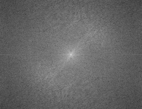
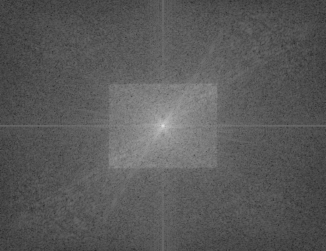
imview(fftshift(log(1+abs(fft(u))))); // display log(1+Fourier-modulus) of the restored image
imview(fftshift(log(1+abs(fft(ref))))); // display log(1+Fourier-modulus) of the reference image
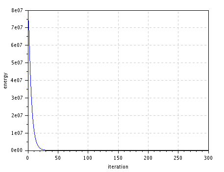
figure(); plot(1:niter,E); // plot energy evolution
xlabel("iteration"); ylabel("energy");
title("Energy decrease");
| reference image | restored image (\(\lambda=0.1\)) |
 |
 |
| Log(1+Fourier-modulus) | Log(1+Fourier-modulus) |
 |
 |
| energy decrease |
 |
Let us resample \(u_0\) over \(\Omega\) using the bicubic spline interpolation.
//* resample u0 over domain Omega using a bicubic spline interpolation *//
x = 0:(nx0-1);
y = 0:(ny0-1);
C = splin2d(y,x,u0,"natural");
xx = linspace(0,nx0-1,nx);
yy = linspace(0,ny0-1,ny);
[XX,YY] = ndgrid(xx,yy);
z_bicubic = (interp2d(YY,XX, y, x, C, "natural"))';
imview(z_bicubic);
imview(fftshift(log(1+abs(fft(z_bicubic))))); // display log(1+Fourier-modulus)
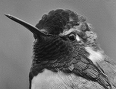
| bicubic spline resampling of \(u_0\) over \(\Omega\) | TV restored image (\(\lambda=0.1\)) |
 |
 |
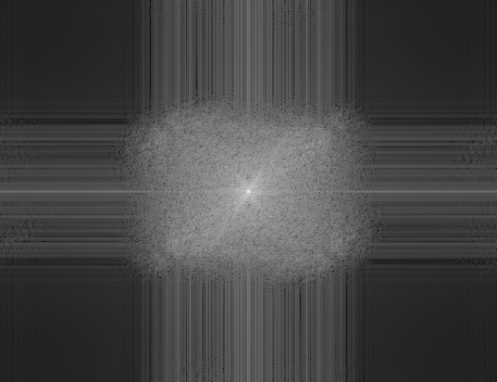
| Log(1+Fourier modulus) | Log(1+Fourier-modulus) |
 |
 |
The image obtained by mean of bicubic interpolation of \(u_0\) is too smooth and presents some ringing artifacts (some edges are replicated into vanishing parallel edges spaced by 2 pixels). Besides, the looking at the modulus of its Fourier transform, we see that the spectrum was completed in a very poor and unrealistic way. The total variation based spectrum extrapolation method yields a better quality image, with a much richer and natural spectrum.
The Huber total variation variant
The use of the discrete total variation as a regularizer for image processing applications has a main drawback, the so-called staircasing effect that is the creation of piecewise constant regions with artificial boundaries in the restored image. This undesirable effect has been rigorously identified and studied in [7,8,9], in particular it is proven (in a more general setting than total variation regularization) in [7] that the non-differentiability at zero of the total variation is responsible of the staircasing artifact.
In order to get rid of the staircasing artifact, we can to replace the \(\ell^2\) norm \(|\cdot|_2\) of the gradient by the Huber-function \(|\cdot|_\alpha\), defined as
\begin{equation} \label{eq:hubernorm} % \forall g \in \RR^2, \quad |g|_\alpha = \left\{ \begin{array}{cl} \frac{|g|_2^2}{2\alpha} & \text{if } |g|_2 \leq \alpha\;, \\ | g |_2 - \frac{\alpha}{2} & \text{otherwise}\;, \end{array} \right. % \end{equation}which is a smooth approximation of the \(\ell^2\)-norm (near \(0\) the \(\ell^2\) norm is being replaced by a quadratic \(\ell^2\) norm).
Given a parameter \(\alpha > 0\), the (discrete) Huber total variation with smoothness parameter \(\alpha\) writes
$$\forall u \in \RR^\Omega, \quad \HTValpha (u) = \sum_{(x,y) \in \Omega} \left| \nabla u (x,y) \right|_\alpha \;, $$
The primal problem
The Huber total variation variant of problem \eqref{eq:primal-inverse} consists in replacing the \(\TV\) regularizer by \(\HTValpha\), the problem writes
\begin{equation} \label{eq:primal-inverse-huber} % \widehat{u}_\text{MAP}^\text{Huber} = \arg\, \min_{u \in \RR^\Omega} \tfrac{1}{2} \| Au - u_0 \|_2^2 + \lambda \HTValpha(u) \;. % \end{equation}Primal-dual formulation
The dual formulation (see the proofs here) of \(\HTValpha\) is given by
\begin{equation*} % \forall u \in \RR^\Omega, \quad \HTValpha(u) = \max_{p \in \RRRR{\Omega}} \langle \nabla u , p \rangle - \tfrac{\alpha}{2} \|p\|_2^2 \quad \text{subject to} \quad \|p\|_{\infty,2} \leq 1 \;, % \end{equation*}replacing accordingly the \(\HTValpha\) term in \eqref{eq:primal-inverse}, and doing as well with the quadratic term \(\tfrac{1}{2}\|Au -u_0\|_2^2\) using \eqref{eq:dual-fidelity}, we get a primal-dual formulation of \eqref{eq:primal-inverse-huber},
\begin{equation} \label{eq:primal-dual-inverse-huber} % \hat{u}_\text{MAP} = \arg \, \min_{u \in \RR^\Omega} \, \max\limits_{\substack{p \in \RRRR{\Omega} \\ q \in \RR^\omega}} \langle \left( \lambda \nabla u , Au \right) , (p,q) \rangle - \delta(p) - \lambda \tfrac{\alpha}{2} \|p\|_2^2 - \tfrac{1}{2} \|q+u_0\|_2^2 \;, % \end{equation}Chambolle-Pock algorithm. Replacing function \(\delta(p)\) by \(\delta(p)+\lambda \tfrac{\alpha}{2} \| p \|_2^2\) into Algorithm 1, leads to a resolvant algorithm for problem \eqref{eq:primal-dual-inverse-huber}. Only the update \eqref{cp.dual-p} corresponding to the dual variable \(p\) is changed, we easily derive a closed-form formula.
Replacing \(\delta(p)\) by \(\delta(p)+\lambda \tfrac{\alpha}{2} \|p\|_2^2\) into Equation \eqref{cp.dual-p}, boils down to the pointwise operations $$ % \forall (x,y) \in \Omega, \quad p^{k+1}(x,y) = \frac{\left(p^k(x,y) + \sigma \lambda \nabla \bar{u}^k(x,y) \right) / \nu }{\max { \left( 1 , \left|\, \left( p^k(x,y) + \sigma \lambda \nabla \bar{u}^k(x,y) \right) / \nu \,\right|_2 \right) }} \;, % $$ where \(\nu = 1+\sigma \alpha \lambda\).
The other updates \eqref{cp.dual-q} and \eqref{cp.primal} are unchanged (see proposition 1).
Scilab implementation. The Scilab implementation is easily adapted to this Huber variant.
function [u,E] = inverse_solver_tvreg_hub(u0,alpha,lambda,niter)

  E = zeros(1,niter);

  // retrieve dimensions of domains omega & Omega (recall
  // that operator A is from R^Omega to R^omega).
  [ny0,nx0] = size(u0);      // domain omega
  [ny,nx] = size(adj_A(u0)); // domain Omega

  // initialize primal and dual variables
  if(exists("init")) then
    if((size(u,1) == ny)&(size(u,2) == nx)) then u = init;
    else u = zeros(ny,nx); end
  else u = zeros(ny,nx); end
  ubar = u;
  px = zeros(u);
  py = zeros(u);
  q = zeros(ny0,nx0);

  // set Chambolle & Pock algorithm time-step parameters
  L = sqrt(8*lambda^2+L_A^2);
  tau = 0.99/L;
  sigma = 0.99/L;
  theta = 1;
  nu = 1+sigma*alpha*lambda;

  //**************************** main loop ****************************//
  for i = 1:niter
    //* compute (Dx,Dy) = grad(ubar) *//
    [Dx,Dy] = grad(ubar);
    //* update p = (px,py) *//
    px  = (px + sigma*lambda*Dx)/nu;
    py  = (py + sigma*lambda*Dy)/nu;
    nrm = px.*px + py.*py;
    id = nrm > 1; nrm = sqrt(nrm(id));
    px(id) = px(id) ./ nrm;
    py(id) = py(id) ./ nrm;
    //* update q *//
    q = (q + sigma*(A(ubar)-u0))/(1+sigma);
    //* compute d = div(p) *//
    d = div(px,py);
    //* update u and ubar *//
    ubar = -theta * u;
    u    = u + tau*(lambda*d-adj_A(q));
    ubar = ubar + (1+theta)*u;
    //* compute energy of u *//
    [Dx,Dy] = grad(u);
    nrm = Dx.^2 + Dy.^2;
    id = (nrm <= alpha^2);
    htv = 0.5/alpha*sum(nrm(id)) + sum(sqrt(nrm(~id))-alpha/2);
    E(i) = 0.5*sum((A(u)-u0).^2) + lambda*htv;
    printf("iteration %d : E = %.10g\n",i,E(i));
  end
  //************************* end of main loop *************************//
endfunction
We briefly test below this algorithm with the three applications studied above. Recall that for each application we must define into Scilab memory the operator \(A\), its adjoint \(A^*\) and an upper bound \(L_A\) of \({|||A|||}\).
Image deconvolution.
//* load blur kernel *//
load('motion_kernel.sod') ; // load the variable "ker" (a motion blur kernel) into Scilab memory...
// ...or define your own kernel, for instance: "ker = ones(5,5)/25;"

//* set operator A = convolution with kernel "ker" *//
function v = A(u)
  v = conv2(u,ker,"valid");
endfunction

//* define the adjoint of A *//
ker_sym = ker($:-1:1,$:-1:1);
function u = adj_A(v)
  u = conv2(v,ker_sym,"full");
endfunction

//* set an upper bound for |||A||| *//
L_A = sum(abs(ker));

//* load the reference image *//
ref = readpgm('fuji.pgm'); // change the path according to the location of the image on your disk.
imview(ref); // display reference image

//* compute a (blurry and noisy) observation u0 *//
sigma = 2;
u0 = A(ref);
u0 = u0 + grand(u0,'nor',0,sigma);
imview(u0); // display u0

//* [optional] choose initial image *//
[ny0,nx0] = size(u0);
dx = floor((size(ker,2)-1)/2);
dy = floor((size(ker,1)-1)/2);
init = u0([ones(1,dy),1:ny0,ny0*ones(1,dy)],[ones(1,dx),1:nx0,nx0*ones(1,dx)]);

//* run algorithms *//
lambda = 0.2; // set regularity parameter
niter = 200; // choose a number of iterations for the Chambolle-Pock algorithm
alpha = 7; // set Huber smoothness parameter
u_iso = inverse_solver_tvreg(u0,lambda,niter);
u_hub = inverse_solver_tvreg_hub(u0,alpha,lambda,niter);
imview(u_iso);
imview(u_hub);

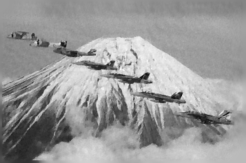
//* crop & zoom outputs (nearest neighbor) *//
imview(u_iso(21:99,1:119).*.ones(3,3));
imview(u_hub(21:99,1:119).*.ones(3,3));
| reference | blurry and noisy (\(\sigma = 2\)) |
 \(~\) \(~\) |
 |
| isotropic \(\TV\) (\(200\) iterations, \(\lambda=0.2\)) | Huber-\(\TV\) (\(200\) iterations, \(\lambda=0.2\), \(\alpha = 7\)) |
 \(~\) \(~\) |
 |
| crop and zoom (\(\times 3\)) | crop and zoom (\(\times 3\)) |
 \(~\) \(~\) |
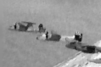 |
Image zooming.
//* set A operator = unzoom with factor z *//
z = 4; // set unzoom factor
function v = A(u)
  [ny,nx] = size(u);
  nx0 = nx/z; // warning: must be an integer
  ny0 = ny/z; // warning: must be an integer
  idx = 1+z*(0:(nx0-1));
  idy = 1+z*(0:(ny0-1));
  v = zeros(ny0,nx0);
  for dx = 0:(z-1)
    for dy = 0:(z-1)
      v = v + u(dy+idy,dx+idx);
    end
  end
  v = v/z^2;
endfunction

//* define the adjoint of A *//
k = ones(z,z)/z^2;
function u = adj_A(v)
  u = v .*. k;
endfunction

//* set an upper bound for |||A||| *//
L_A = 1/z;

//* open reference image *//
ref = readpgm('eye.pgm'); // change the path according to the location of the image on your disk.
imview(ref); // display reference image

//* compute an observation u0 *//
sigma = 2;
u0 = A(ref);
u0 = u0 + grand(u0,'nor',0,sigma);
imview(u0);

//* run algorithms *//
niter = 2000;
lambda = 0.2;
alpha = 7; // set Huber smoothness parameter
init = u0.*.ones(z,z); // set init = nearest neighbor zoom of factor z of u0.
u_iso = inverse_solver_tvreg(u0,lambda,niter);
u_hub = inverse_solver_tvreg_hub(u0,alpha,lambda,niter);
imview(init); // display details of u0
imview(u_iso); // display isotropic-TV restored image
imview(u_hub); // display Huber-TV restored image
| reference / \(u_0\) | details of \(u_0\) (nearest-neighbor zoom of \(u_0\)) |
 \(~\) \(~\) |
 |
| isotropic \(\TV\) (\(2000\) iterations, \(\lambda=0.2\)) | Huber-\(\TV\) (\(2000\) iterations, \(\lambda=0.2\), \(\alpha = 7\)) |
 \(~\) \(~\) |
 |
Spectrum extrapolation.
//* load the reference image *//
ref = readpgm('hummingbird.pgm'); // change the path according to the location of the image on your disk.

//* precompute Omega and omega dimensions *//
z = 3; // set the square root of the ratio |Omega|/|omega|
[ny,nx] = size(ref);
nx0 = round(nx/z);
ny0 = round(ny/z);

//* ensures omega has odd x odd dimensions *//
if(modulo(nx0,2)==0) then nx0 = nx0-1; end
if(modulo(ny0,2)==0) then ny0 = ny0-1; end
z = sqrt((nx*ny)/(nx0*ny0)); // update sqrt(|Omega|/|omega|)


//* define omega_x, omega_y = indexes of frequencies omega into Omega. *//
//* this allows to restrict the Fourier domain Omega to omega.         *//
omega_x = 1+modulo(nx + ifftshift((0:nx0-1)-floor(nx0/2)), nx);
omega_y = 1+modulo(ny + ifftshift((0:ny0-1)-floor(ny0/2)), ny);

//* define operator A *//
function v = A(u)
  dft_u = fft(u);
  dft_v = dft_u(omega_y,omega_x);
  v = 1/z^2 * real(ifft(dft_v));
endfunction

//* define the adjoint of A *//
function u = adj_A(v)
  dft_u = zeros(ny,nx);
  dft_u(omega_y,omega_x) = fft(v);
  u = real(ifft(dft_u));
endfunction

//* set an upper bound for |||A||| *//
L_A = 1;

//* compute an observation u0 *//
sigma = 2; // set the level of noise
u0 = A(ref) + grand(ny0,nx0,'nor',0,sigma);
imview(ref); // display reference image
imview(u0); // display observed image

//* run algorithms *//
alpha = 5; // set Huber smoothness parameter
lambda = 0.1;
niter = 300;
clear init; // we will use default initializer (null image)
u_iso = inverse_solver_tvreg(u0,lambda,niter);
u_hub = inverse_solver_tvreg_hub(u0,alpha,lambda,niter);
imview(u_iso); // display isotropic-TV restored image
imview(u_hub); // display Huber-TV restored image
| reference image | observed image \(u_0\) (\(\sigma=2\)) |
 |
 |
| isotropic \(\TV\) (\(300\) iterations, \(\lambda=0.1\)) | Huber-\(\TV\) (\(300\) iterations, \(\lambda=0.1\), \(\alpha = 5\)) |
 \(~\) \(~\) |
 |
References
- Rudin, L. I., Osher, S., and Fatemi, E.: ``Nonlinear total variation based noise removal algorithms'', Physica D 60(1), pp. 259–268, 1992.
- Ekeland, I., and Témam, R.: ``Convex analysis and variational problems'', volume 28 of Classics in Applied Mathematics. Society for Industrial and Applied Mathematics (SIAM), Philadelphia, PA, english edition, 1999. Translated from the French.
- Chambolle, A., Pock, T.: ``A first-order primal-dual algorithm for convex problems with applications to imaging'', Journal of Mathematical Imaging and Vision, vol. 40, pp. 120–145, 2011.
- Chambolle, A., Caselles, V., Cremers, D., Novaga, M., and Pock, T.: `` An introduction to total variation for image analysis'', Theoretical foundations and numerical methods for sparse recovery, 9, 263–340, 2010.
- Guichard, F., and Malgouyres, F.: ``Total variation based interpolation'', In Proceedings of the European signal processing conference, vol. 3, pp. 1741–1744, 1998.
- Malgouyres, F., and Guichard, F.: ``Edge direction preserving image zooming: a mathematical and numerical analysis'', SIAM Journal on Numerical Analysis, vol. 39(1), pp. 1–37, 2001.
- Nikolova, M.: ``Local Strong Homogeneity of a Regularized Estimator'', SIAM Journal on Applied Mathematics, vol. 61, pp. 633–658, 2000.
- Chan, T. F., Marquina, A., and Mulet, P.: ``Higher Order Total Variation-Based Image Restoration'', SIAM Journal on Scientific Computing, vol. 22, pp. 503–516, 2000.
- Ring, W.: ``Structural Properties of Solutions to Total Variation Regularization Problems'', M2AN, Modélisation Mathématique et Analyse Numérique, vol. 34, pp. 799–810, 2000.